Variational Autoencoders
Variational Autoencoders (VAEs) combine the power of neural networks with probabilistic inference to model complex data distributions. This blog unpacks the intuition, math, and implementation of VAEs — from KL divergence and the ELBO to PyTorch code that generates to generate new images.
1 Autoencoders vs Variational Autoencoders
Traditional autoencoders learn to compress data into a lower-dimensional representation (latent space) and reconstruct it. However, they fall short in several areas:
- They lack generative capabilities — they cannot sample new data effectively
- The latent space is unstructured, offering little control or interpretation
- There is no probabilistic modeling, limiting uncertainty estimation
Variational Autoencoders (VAEs) were introduced to overcome these limitations. Rather than encoding inputs into fixed latent vectors, VAEs learn a probabilistic latent space by modeling each input as a distribution — typically a Gaussian with a learned mean \(\\mu\) and standard deviation \(\\sigma\). This approach enables the model to sample latent variables \(z\) using the reparameterization trick, allowing the entire architecture to remain differentiable and trainable. By doing so, VAEs not only enable reconstruction, but also promote the learning of a continuous, interpretable latent space — a key enabler for generation and interpolation.
The diagram below illustrates this process:

Source: Wikimedia Commons, licensed under CC BY-SA 4.0.
2 Probabilistic Framework
More formally, VAEs assume the data is generated by a two-step process:
- Sample a latent variable \(\mathbf{z} \sim \mathcal{N}(0, I)\)
- Generate the observation \(\mathbf{x}\) from: \[ p(\mathbf{x}|\mathbf{z}) = \mathcal{N}(\mu_\theta(\mathbf{z}), \Sigma_\theta(\mathbf{z})) \] where \(\mu_\theta\) and \(\Sigma_\theta\) are neural networks parameterized by \(\theta\)
Here, \(\mathbf{z}\) acts as a hidden or latent variable, which is unobserved during training. The model thus defines a mixture of infinitely many Gaussians — one for each \(\mathbf{z}\).
To compute the likelihood of a data point \(\mathbf{x}\), we must marginalize over all possible latent variables: \[ p(\mathbf{x}) = \int p(\mathbf{x}, \mathbf{z}) \, d\mathbf{z} \]
This integral requires integrating over all possible values of the latent variable \(\mathbf{z}\), which is often high-dimensional and affects the likelihood in a non-linear way through neural networks. Because of this, computing the marginal likelihood exactly is computationally intractable. This motivates the use of techniques like variational inference and ELBO.
2.1 Computational Challenge
This integral requires integrating over:
- All possible values of \(\mathbf{z}\) (often high-dimensional)
- Non-linear transformations through neural networks
Result: Exact computation is intractable, motivating techniques like variational inference and ELBO (developed next).
3 Estimating the Marginal Likelihood
3.1 Naive Monte Carlo Estimation
One natural idea is to approximate the integral using samples from a simple distribution like the uniform distribution:
\[ p(x) \approx \frac{1}{K} \sum_{j=1}^K p_\theta(x, z_j), \quad z_j \sim \text{Uniform} \]
However, this fails in practice. For most values of \(z\), the joint probability \(p_\theta(x, z)\) is very low. Only a small region of the latent space contributes significantly to the integral. Since uniform sampling does not concentrate around these regions, the estimator has high variance and rarely “hits” likely values of \(z\).
3.2 Importance Sampling
To address this, we use importance sampling, introducing a proposal distribution \(q(z)\):
\[ p(x) = \mathbb{E}_{q(z)} \left[ \frac{p_\theta(x, z)}{q(z)} \right] \]
This gives an unbiased estimator of \(p(x)\) if \(q(z)\) is well-chosen (ideally close to \(p_\theta(z|x)\)). Intuitively, we sample \(z\) more frequently in regions where \(p_\theta(x, z)\) is high.
3.3 Log likelihood
Our goal is to optimize the log-likelihood, and the log of an expectation is not the same as the expectation of the log. That is,
\[ \log p(x) = log \mathbb{E}_{q(z)} \left[ \frac{p_\theta(x, z)}{q(z)} \right] \neq \mathbb{E}_{q(z)} \left[ \log \frac{p_\theta(x, z)}{q(z)} \right] \]
While the marginal likelihood p(x) can be estimated unbiasedly using importance sampling, estimating its logarithm \(p(x)\) introduces bias due to the concavity of the log function. This is captured by Jensen’s Inequality, which tells us:
\[ \log \mathbb{E}_{q(z)} \left[ \frac{p_\theta(x, z)}{q(z)} \right] \geq \underbrace{\mathbb{E}_{q(z)} \left[ \log \frac{p_\theta(x, z)}{q(z)} \right]}_{\text{ELBO}} \]
This means that the expected log of the estimator underestimates the true log-likelihood. The right-hand side provides a tractable surrogate objective known as the Evidence Lower Bound (ELBO), which is a biased lower bound to \(\log p(x)\). Optimizing the ELBO allows us to indirectly maximize the intractable log-likelihood.
In the next section, we formally derive this bound and explore its components in detail.
4 Why Variational Inference?
Computing the true posterior distribution \(p(z \mid x)\) is intractable in most cases, because it requires evaluating the marginal likelihood \(p(x)\), which involves integrating over all possible values of \(z\):
\[ p(x) = \int p(x, z) \, dz \]
Variational inference tackles this by introducing a tractable, parameterized distribution \(q(z)\) to approximate \(p(z|x)\). We aim to make \(q(z)\) as close as possible to the true posterior by minimizing the KL divergence:
\[ D_{\text{KL}}(q(z) \| p(z|x)) \]
This turns inference into an optimization problem. A key result is the Evidence Lower Bound (ELBO). See next section.
5 Training a VAE
5.1 ELBO Objective
Now that we’ve introduced the challenge of approximating the intractable posterior using variational inference, we turn our attention to deriving the Evidence Lower Bound (ELBO). This derivation reveals how optimizing a surrogate objective allows us to approximate the true log-likelihood of the data while keeping the approximate posterior close to the prior. The steps below walk through this formulation.
5.1.1 KL Divergence Objective
\[\begin{equation} D_{KL}(q(z)\|p(z|x; \theta)) = \sum_z q(z) \log \frac{q(z)}{p(z|x; \theta)} \end{equation}\]
5.1.2 Apply Bayes’ Rule
Substitute \(p(z|x; \theta) = \frac{p(z,x;\theta)}{p(x;\theta)}\): \[\begin{equation} = \sum_z q(z) \log \left( \frac{q(z) \cdot p(x; \theta)}{p(z, x; \theta)} \right) \end{equation}\]
5.1.3 Decompose Terms
\[\begin{align} &= \sum_z q(z) \log q(z) + \sum_z q(z) \log p(x; \theta) \nonumber \\ &\quad - \sum_z q(z) \log p(z, x; \theta) \\ &= -H(q) + \log p(x; \theta) - \mathbb{E}_q[\log p(z,x;\theta)] \end{align}\]
Note: The term \(\mathcal{H}(q)\) represents the entropy of the variational distribution \(q(z|x)\). Entropy is defined as:
\[ \mathcal{H}(q) = -\sum_z q(z) \log q(z) = -\mathbb{E}_{q(z)}[\log q(z)] \]
Entropy measures the amount of uncertainty or “spread” in a distribution. A high-entropy \(q(z)\) places probability mass across a wide region of the latent space, while a low-entropy \(q(z)\) is more concentrated. This decomposition is key to understanding the KL divergence term in the ELBO.
5.1.4 Rearrange for ELBO
\[ \log p(x; \theta) = \underbrace{ \mathbb{E}_q[\log p(z, x; \theta)] + \mathcal{H}(q) }_{\text{ELBO}} +D_{KL}(q(z)\|p(z|x; \theta)) \]
This equation shows that the log-likelihood \(\log p(x)\) can be decomposed into the ELBO and the KL divergence between the approximate posterior and the true posterior. Since the KL divergence is always non-negative, the ELBO serves as a lower bound to the log-likelihood. By maximizing the ELBO, we indirectly minimize the KL divergence, bringing \(q(z)\) closer to \(p(z|x)\).
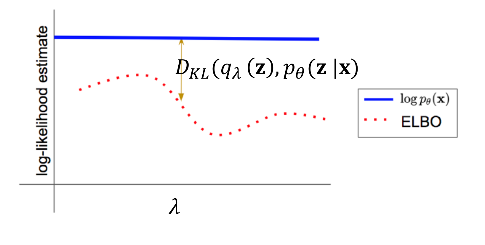 Visualizing how \(\log p(x)\) decomposes into the ELBO and KL divergence.
Source: deepgenerativemodels.github.io
5.1.5 Key Results
Evidence Lower Bound (ELBO): \[\begin{equation} \mathcal{L}(\theta,\phi) = \mathbb{E}_{q(z;\phi)}[\log p(x,z;\theta)] + H(q(z;\phi)) \end{equation}\]
Optimization: \[\begin{equation} \max_{\theta,\phi} \mathcal{L}(\theta,\phi) \Rightarrow \begin{cases} \text{Maximizes data likelihood} \\ \text{Minimizes } D_{KL}(q\|p) \end{cases} \end{equation}\]
6 Understanding the KL Divergence Term in the VAE Loss
In a VAE, the KL divergence term penalizes the encoder for producing latent distributions that deviate too far from the standard normal prior. This regularization has several important benefits:
- It ensures that the latent space has a consistent structure, enabling meaningful sampling and interpolation.
- It helps avoid large gaps between clusters in latent space by encouraging the encoder to distribute representations more uniformly.
- It pushes the model to use the space around the origin more symmetrically and efficiently.
6.1 Balancing KL Divergence and Reconstruction
In a Variational Autoencoder, the loss balances two goals:
- Reconstruction — making the output resemble the input
- Regularization — keeping the latent space close to a standard normal distribution
This is captured by the loss function:
\[ \mathcal{L}_{\text{VAE}} = \text{Reconstruction Loss} + \beta \cdot D_{\text{KL}}(q(z|x) \,\|\, p(z)) \]
The parameter \(\beta\) controls how strongly we enforce this regularization. Getting its value right is critical.
6.1.1 When \(\beta\) is too low:
- The model mostly ignores the KL term, behaving like a plain autoencoder
- The latent space becomes disorganized or fragmented
- Sampling from the prior \(p(z) = \mathcal{N}(0, I)\) results in unrealistic or broken outputs
6.1.2 When \(\beta\) is too high:
- The encoder is forced to keep \(q(z|x)\) too close to the prior
- It encodes less information about the input
- Reconstructions become blurry or generic, since the decoder gets little to work with
Choosing \(\beta\) carefully is essential for balancing generalization and fidelity.
A well-tuned \(\beta\) helps the VAE both reconstruct accurately and generate new samples that resemble the training data.
6.2 Gradient Challenge
In variational inference, we approximate the true posterior \(p(z|x)\) with a tractable distribution \(q_\phi(z)\). This allows us to optimize the ELBO:
\[ \mathcal{L}(x; \theta, \phi) = \mathbb{E}_{q(z; \phi)} \left[ \log p(z, x; \theta) - \log q(z; \phi) \right] \]
Our goal is to maximize this objective with respect to both \(\theta\) and \(\phi\). While computing the gradient with respect to \(\theta\) is straightforward, optimizing with respect to \(\phi\) presents a challenge.
The complication arises because \(\phi\) appears both in the density \(q_\phi(z|x)\) and in the expectation operator. That is:
\[ \nabla_\phi \mathbb{E}_{q(z; \phi)} \left[ \log p(z, x; \theta) - \log q(z; \phi) \right] \]
This gradient is hard to compute directly because we’re sampling from a distribution that depends on the parameters we’re trying to update.
6.3 The Reparameterization Trick
To make this expression differentiable, we reparameterize the random variable \(z\) as a deterministic transformation of a parameter-free noise variable \(\epsilon\):
\[ \epsilon \sim \mathcal{N}(0, I), \quad z = \mu_\phi(x) + \sigma_\phi(x) \cdot \epsilon \]
This turns the expectation into:
\[ \mathbb{E}_{\epsilon \sim \mathcal{N}(0, I)}\left[ \log p(z, x; \theta) - \log q(z; \phi) \right] \]
where \(z\) is now a differentiable function of \(\phi\).

Image source: Wikipedia (CC BY-SA 4.0)
This diagram illustrates how the reparameterization trick enables differentiable sampling:
- In the original formulation, \(z\) is sampled directly from a learned distribution, breaking the gradient flow.
- In the reparameterized formulation, we sample noise \(\epsilon \sim \mathcal{N}(0, I)\), and compute \(z = \mu + \sigma \cdot \epsilon\), making the sampling path fully differentiable.
6.3.1 Monte Carlo Approximation
We approximate the expectation using Monte Carlo sampling:
\[ \mathbb{E}_{\epsilon}[\log p_\theta(x, z) - \log q_\phi(z)] \approx \frac{1}{K} \sum_{k=1}^K \left[\log p_\theta(x, z^{(k)}) - \log q_\phi(z^{(k)})\right] \]
with:
\[ z^{(k)} = \mu_\phi(x) + \sigma_\phi(x) \cdot \epsilon^{(k)}, \quad \epsilon^{(k)} \sim \mathcal{N}(0, I) \]
This enables us to compute gradients using backpropagation.
6.3.2 Summary
- Variational inference introduces a gradient challenge because \(q_\phi(z)\) depends on \(\phi\)
- The reparameterization trick expresses \(z\) as a differentiable function of noise and \(\phi\)
- This allows us to use backpropagation to optimize the ELBO efficiently
6.4 Amortized Inference
In classical variational inference, we introduce a separate set of variational parameters \(\phi^i\) for each datapoint \(x^i\) to approximate the true posterior \(p(z|x^i)\). However:
Optimizing a separate \(\phi^i\) for every datapoint is computationally expensive and does not scale to large datasets.
6.4.1 The Key Idea: Amortization
Instead of learning and storing a separate \(\phi^i\) for every datapoint, we learn a single parametric function \(f_\phi(x)\) — typically a neural network — that maps each input \(x\) to the parameters of the approximate posterior:
\[ q_\phi(z|x) = \mathcal{N}\left(\mu_\phi(x), \sigma^2_\phi(x)\right) \]
Here, \(\phi\) are the shared parameters of the encoder network, and \(\mu_\phi(x), \sigma_\phi(x)\) are its outputs.
This is like learning a regression function that predicts the optimal variational parameters for any input \(x\).
6.5 Training with Amortized Inference
Our training objective remains the ELBO:
\[ \mathcal{L}(x; \theta, \phi) = \mathbb{E}_{q_\phi(z|x)}\left[\log p_\theta(x, z) - \log q_\phi(z|x)\right] \]
We optimize both \(\theta\) (decoder parameters) and \(\phi\) (encoder parameters) using stochastic gradient descent.
6.5.1 Algorithm:
Initialize \(\theta^{(0)}, \phi^{(0)}\)
Sample a datapoint \(x^i\)
Use \(f_\phi(x^i)\) to produce \(\mu^i, \sigma^i\)
Sample \(z^i = \mu^i + \sigma^i \cdot \epsilon\), with \(\epsilon \sim \mathcal{N}(0, I)\)
Estimate the ELBO and compute gradients w.r.t. \(\theta, \phi\)
Update \(\theta, \phi\) using gradient descent
Update \(\theta\), \(\phi\) using gradient descent:
\[ \phi \leftarrow \phi + \tilde{\nabla}_\phi \sum_{x \in \mathcal{B}} \text{ELBO}(x; \theta, \phi) \]
\[ \theta \leftarrow \theta + \tilde{\nabla}_\theta \sum_{x \in \mathcal{B}} \text{ELBO}(x; \theta, \phi) \]
where \(\mathcal{B}\) is the current minibatch and \(\tilde{\nabla}\) indicates a stochastic gradient approximation.
6.6 Summary
- Amortized inference replaces per-datapoint optimization with a single learned mapping \(f_\phi(x)\)
- This makes variational inference scalable and efficient
- The model can generalize to unseen inputs by predicting variational parameters on-the-fly
Note: Following common practice in the literature, we use \(\phi\) to denote the parameters of the encoder network, even though it now defines a function rather than individual variational parameters.
7 Applications of VAEs
Variational Autoencoders are widely used in:
- Image Generation: VAEs can generate new images similar to the training data (e.g., MNIST digits)
- Anomaly Detection: High reconstruction error flags unusual data points
- Representation Learning: Latent space captures features for downstream tasks
7.1 😎 Face Generation with Convolutional VAE
To complement the theory, I’ve built a full PyTorch implementation of a Variational Autoencoder trained on the CelebA dataset.
📘 The notebook walks through:
- Defining the encoder, decoder, and reparameterization trick
- Implementing the ELBO loss function (reconstruction + KL divergence)
- Training the model on face images
- Generating new faces from random latent vectors
8 This example is designed to reinforce the theoretical concepts from earlier sections.
9 Further Reading
For readers interested in diving deeper into the theory and applications of variational autoencoders, the following resources are recommended:
Tutorial on Variational Autoencoders
Carl Doersch (2016)
https://arxiv.org/pdf/1606.05908Auto-Encoding Variational Bayes
Kingma & Welling (2014) — the original VAE paper
https://arxiv.org/pdf/1312.6114The Challenges of Amortized Inference for Structured Prediction
Cremer, Li, & Duvenaud (2019)
https://arxiv.org/pdf/1906.02691Deep Generative Models course notes
https://deepgenerativemodels.github.io/notes/vae/