Energy Based Models (EBM)
1 Introduction
Modern generative models impose strict architectural requirements:
- VAEs need encoder-decoder pairs
- GANs require adversarial networks
- Normalizing flows must use invertible transforms
While each model family has strengths, they also carry trade-offs:
- VAEs often produce blurry samples due to reliance on Gaussian assumptions.
- GANs can generate high-quality images but are notoriously unstable and suffer from mode collapse.
- Normalizing Flows guarantee exact likelihoods but restrict architecture design due to invertibility constraints.
Energy-Based Models (EBMs) break this pattern by:
Learning a scoring function (energy) where it assigns low energy to likely or observed data (\(x \sim p_{data}\)), and high energy to unlikely or unobserved inputs.
Linking to probability via: \(p_\theta(x) = \frac{e^{-E_\theta(x)}}{Z(\theta)}, \quad Z(\theta) = \int e^{-E_\theta(x)}\,dx\)
where low energy = high probability
Using generic neural nets—no specialized architectures needed
This approach provides unique advantages:
✓ Simpler setup - works with any neural net
✓ Explicit scoring - \(p(x) \propto e^{-E(x)}\) (energy)
✓ Stable training - No adversarial balancing act like GANs
EBMs replace architectural constraints with a single principle:
“Learn to distinguish real data from noise through energy scoring.”
To understand how this works mathematically, we must first answer: What defines a valid probability distribution?
The next section derives EBMs’ theoretical foundation—revealing how they bypass traditional limitations while introducing new challenges (like partition function estimation).
2 Math Review
2.1 Understanding the Probability Foundation Behind EBMs
In generative modeling, a valid probability distribution \(p(x)\) must satisfy:
Non-negativity:
\[ p(x) \geq 0 \]Normalization:
\[ \int p(x)\, dx = 1 \]
While it’s easy to define a function that satisfies \(p(x) \geq 0\) (e.g., using exponentials), ensuring that it also sums to 1 — i.e., \(\int p(x)\, dx = 1\) — is much more difficult, especially for flexible functions like neural networks.
2.2 Why do we introduce \(g(x)\)?
Instead of modeling \(p(x)\) directly, we define a non-negative function \(g(x) \geq 0\) and turn it into a probability distribution by normalizing:
\[ p_\theta(x) = \frac{g_\theta(x)}{Z(\theta)}, \quad \text{where} \quad Z(\theta) = \int g_\theta(x)\, dx \]
This trick simplifies the problem by separating the two requirements:
- \(g_\theta(x)\) ensures non-negativity
- \(Z(\theta)\) enforces normalization
The normalization constant \(Z(\theta)\) is also known as the partition function.
This trick allows us to use any expressive function for \(g_\theta(x)\) — including deep neural networks.
2.2.1 Intuition
Think of \(g_\theta(x)\) as a scoring function:
- Higher \(g_\theta(x)\) means more likely
- Dividing by \(Z(\theta)\) rescales these scores to form a valid probability distribution
2.3 Energy-Based Parameterization
We’ve just seen how \(g_\theta(x)\) can be any non-negative function. A common and powerful choice is to define it using an exponential transformation:
\[ g_\theta(x) = \exp(f_\theta(x)) \]
This ensures that \(g_\theta(x) \geq 0\) and allows us to interpret \(f_\theta(x)\) as an unnormalized log-probability score.
We then normalize using the partition function ( Z() ) to obtain a valid probability distribution:
\[ p_\theta(x) = \frac{g_\theta(x)}{Z(\theta)} = \frac{\exp(f_\theta(x))}{Z(\theta)}, \quad \text{where} \quad Z(\theta) = \int \exp(f_\theta(x)) \, dx \]
This leads to the energy-based formulation, where \(f_\theta(x)\) is interpreted as the negative energy. We can equivalently write:
\[ E_\theta(x) = -f_\theta(x) \quad \Rightarrow \quad p_\theta(x) = \frac{\exp(-E_\theta(x))}{Z(\theta)} \]
Energy-Based Models (EBMs) follow this foundational idea: define a scoring function \(f_\theta(x)\) that assigns high values to likely data points, then convert those scores into probabilities using exponentiation and normalization.
This perspective offers four key advantages:
- It allows us to use flexible models (like deep neural networks) to assign unnormalized scores.
- It separates concerns: one function ensures non-negativity (via exponentiation), and the partition function enforces normalization.
- It lets us interpret \(f_\theta(x)\) as an unnormalized log-probability, improving interpretability.
- It connects naturally to well-known distributions (e.g., exponential family, Boltzmann distribution), making the formulation more general.
This formulation gives us the freedom to model complex distributions with any differentiable scoring function \(f_\theta(x)\), while only requiring that we can compute or approximate its gradients.
2.3.1 Summary
Whether we express scores directly via \(f_\theta(x)\) or indirectly through energy \(E_\theta(x)\), the core idea remains the same:
- Use a flexible model to assign unnormalized scores
- Normalize those scores using the partition function \(Z(\theta)\)
This gives EBMs the freedom to model complex data distributions using any differentiable function for \(f_\theta(x)\) — without requiring invertibility or exact likelihoods.
2.3.2 Visualizing Energy Functions
Let’s now build visual intuition for what these energy landscapes look like.
Energy-based models capture compatibility between variables using an energy function. In this example (adapted from Atcold, 2020), the energy function assigns lower values to pairs of variables \((x, y)\) that are more likely to co-occur — and higher energy elsewhere.
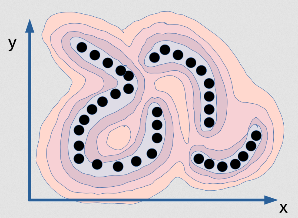
Visualizing the energy landscape \(E(x_1, x_2)\) — lower energy corresponds to higher probability.
This shows how EBMs encode knowledge: valleys indicate high-likelihood (real) data, while peaks represent unlikely (noise) regions.
This kind of energy landscape is especially useful in practical tasks like image generation, where the model learns to assign low energy to realistic images and high energy to unrealistic ones. During inference, the model can generate new samples by exploring low-energy regions of this landscape.
3 Practical Applications
Energy-Based Models (EBMs) offer unique benefits in scenarios where traditional models struggle. Below are two practical applications that demonstrate how EBMs shine in real-world settings.
3.1 When You Don’t Need the Partition Function
In general, evaluating the full probability \(p_\theta(x)\) requires computing the partition function \(Z(\theta)\):
\[ p_\theta(x) = \frac{1}{Z(\theta)} \exp(f_\theta(x)) \]
Key Insight
In some applications, we don’t need the exact probability — we only need to compare scores. This allows EBMs to be useful even when the partition function is intractable.
When comparing two samples \(x\) and \(x'\), we can compute the ratio of their probabilities:
\[ \frac{p_\theta(x)}{p_\theta(x')} = \exp(f_\theta(x) - f_\theta(x')) \]
This lets us determine which input is more likely — without ever computing \(Z(\theta)\) — a powerful advantage of EBMs.
Practical Applications:
- Anomaly detection: Identify inputs with unusually low likelihood.
- Denoising: Prefer cleaner versions of corrupted data by comparing likelihoods.
- Object recognition: Assign the most likely label to an input image.
- Sequence labeling: Predict tags (e.g., part-of-speech) for input tokens.
- Image restoration: Recover clean images from noisy inputs.
Real-World Example
In anomaly detection, EBMs have been used to identify outliers in high-dimensional sensor data without computing exact probabilities — simply by scoring input configurations and flagging those with unusually high energy.
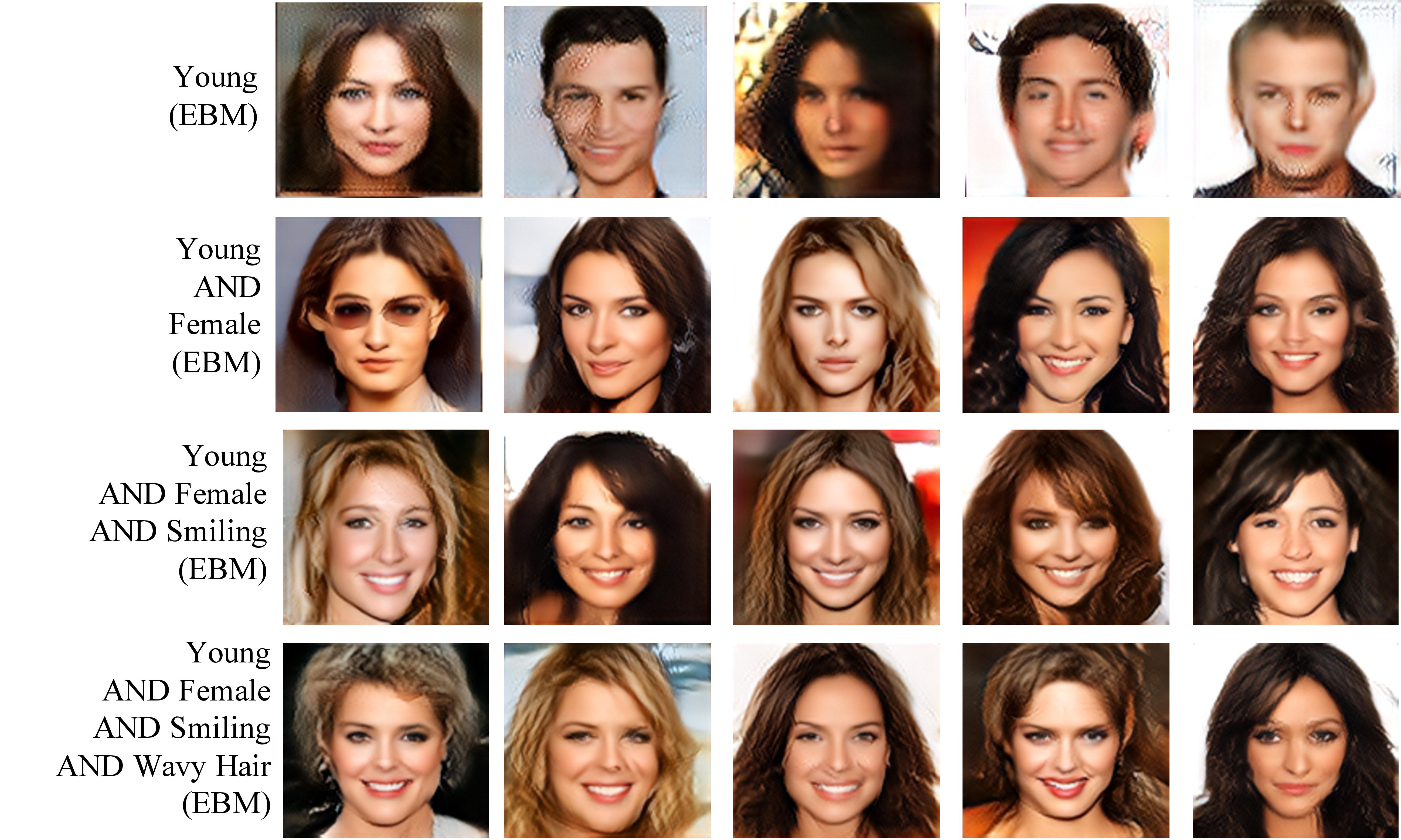
3.2 Product of Experts (Compositional Generation)
In some cases, we want to combine multiple expert models that each score different attributes of an input \(\mathbf{x}\) — for example, age, gender, or hairstyle. This is where Energy-Based Models (EBMs) shine through Product of Experts (PoE).
Suppose you have three trained expert models \(f_{\theta_1}(x)\), \(f_{\theta_2}(x)\), and \(f_{\theta_3}(x)\). A tempting idea is to combine their scores additively and exponentiate:
\[ \exp\left(f_{\theta_1}(x) + f_{\theta_2}(x) + f_{\theta_3}(x)\right) \]
To make this a valid probability distribution, we normalize:
\[ p_{\theta_1, \theta_2, \theta_3}(x) = \frac{1}{Z(\theta_1, \theta_2, \theta_3)} \exp\left(f_{\theta_1}(x) + f_{\theta_2}(x) + f_{\theta_3}(x)\right) \]
This behaves like a logical AND: if any expert assigns low score, the overall likelihood drops. This contrasts with mixture models (like Mixture of Gaussians), which behave more like OR.
Real-World Example
In the figure below (Du et al., 2020), EBMs were used to model attributes like “young”, “female”, “smiling”, and “wavy hair”. By combining these via Product of Experts, the model generated faces that satisfied multiple specific attributes simultaneously.
4 Benefits and Limitations of EBMs
4.1 Key Benefits
Very flexible model architectures
No need for invertibility, autoregressive factorization, or adversarial design.
Stable training
Compared to GANs, EBMs can be more robust and easier to optimize.
High sample quality
Capable of modeling complex, multi-modal data distributions.
Flexible composition
Energies can be combined to support multi-task objectives or structured learning.
4.2 Limitations
Despite their strengths, EBMs come with notable challenges:
Sampling is expensive
No direct way to sample from \(p_\theta(x)\); MCMC methods are slow and scale poorly.
Likelihood is intractable
Partition function \(Z(\theta)\) is hard to compute, and we can’t directly evaluate log-likelihood.
Training is indirect
Learning requires reducing energy of incorrect samples, not just increasing for correct ones.
No feature learning (by default)
EBMs don’t learn latent features unless explicitly structured (e.g., RBMs).
5 Training Energy-Based Models
EBMs are trained to assign higher scores (lower energy) to observed data points, and lower scores (higher energy) to unobserved ones. This corresponds to maximizing the likelihood of training data.
\[ p_\theta(x_{\text{train}}) = \frac{\exp(f_\theta(x_{\text{train}}))}{Z(\theta)} \]
This expression tells us that increasing the score for \(x_{\text{train}}\) is not enough — we must also decrease scores for other \(x\) to reduce \(Z(\theta)\) and make the probability higher relatively.
5.1 Log-Likelihood and Its Gradient
To train EBMs, we compute the gradient of the log-likelihood with respect to parameters \(\theta\).
We start by writing the log-likelihood:
\[ \log p_\theta(x_{\text{train}}) = f_\theta(x_{\text{train}}) - \log Z(\theta) \]
Taking the gradient with respect to \(\theta\):
\[ \nabla_\theta \log p_\theta(x_{\text{train}}) = \nabla_\theta f_\theta(x_{\text{train}}) - \nabla_\theta \log Z(\theta) \]
To compute this, we need the gradient of the log partition function:
\[ Z(\theta) = \int \exp(f_\theta(x))\, dx \]
Applying the chain rule:
\[ \nabla_\theta \log Z(\theta) = \frac{1}{Z(\theta)} \int \exp(f_\theta(x)) \nabla_\theta f_\theta(x)\, dx = \mathbb{E}_{x \sim p_\theta} \left[ \nabla_\theta f_\theta(x) \right] \]
Substitute this back:
\[ \nabla_\theta \log p_\theta(x_{\text{train}}) = \nabla_\theta f_\theta(x_{\text{train}}) - \mathbb{E}_{x \sim p_\theta} \left[ \nabla_\theta f_\theta(x) \right] \]
The first term is straightforward — it’s the gradient of the model’s score on the training point.
But the second term, the expectation over model samples, is difficult. It requires drawing samples from \(p_\theta(x)\), which in turn depends on the intractable normalization constant \(Z(\theta)\).
To deal with this, we use sampling-based approximations like Contrastive Divergence.
5.2 Contrastive Divergence
Since computing the true gradient requires sampling from \(p_\theta(x)\), which is intractable due to the partition function \(Z(\theta)\), we use Contrastive Divergence as an efficient approximation.
We approximate the expectation:
\[ \mathbb{E}_{x \sim p_\theta} \left[ \nabla_\theta f_\theta(x) \right] \approx \nabla_\theta f_\theta(x_{\text{sample}}) \]
This gives:
\[ \nabla_\theta \log p_\theta(x_{\text{train}}) \approx \nabla_\theta f_\theta(x_{\text{train}}) - \nabla_\theta f_\theta(x_{\text{sample}}) = \nabla_\theta \left( f_\theta(x_{\text{train}}) - f_\theta(x_{\text{sample}}) \right) \]
Contrastive Divergence Algorithm:
- Sample \(x_{\text{sample}} \sim p_\theta\) (typically via MCMC)
- Take a gradient step on:
\[ \nabla_\theta \left( f_\theta(x_{\text{train}}) - f_\theta(x_{\text{sample}}) \right) \]
This encourages the model to increase the score of the training sample and decrease the score of samples it currently believes are likely.
EBM Training Recap
- Want: High scores (low energy) for real data
- Avoid: High scores for incorrect data
- Can’t compute exact gradient due to \(Z(\theta)\)
- So: Approximate using Monte Carlo sample \(\sim p_\theta(x)\)
5.2.1 Intuition Recap
- Pull up: Increase the score (lower the energy) of the real training sample \(\nabla_\theta f_\theta(x_{\text{train}})\)
- Push down: Decrease the score of samples from the model \(\nabla_\theta f_\theta(x_{\text{sample}})\)
- This sharpens the model’s belief in real data and corrects high-scoring regions where it is currently overconfident.
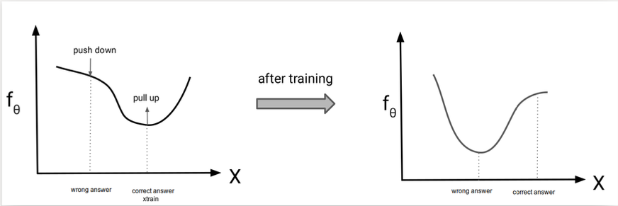 During training, EBMs increase the score of correct samples and decrease the score of incorrect ones.
Source: course material from CS236: Deep Generative Models
6 Sampling from Energy-Based Models
Recall that EBMs define a probability distribution as:
\[ p_\theta(x) = \frac{1}{Z(\theta)} \exp(f_\theta(x)) \]
Unlike autoregressive or flow models, there is no direct way to sample from \(p_\theta(x)\) because we cannot easily compute how likely each possible sample is. That’s because the normalization term \(Z(\theta)\) is intractable.
However, we can still compare two samples using a key insight:
Key Insight
We can still compare two samples \(x\) and \(x'\) without needing \(Z(\theta)\):
\[ \frac{p_\theta(x)}{p_\theta(x')} = \exp(f_\theta(x) - f_\theta(x')) \]
This property is useful for tasks like ranking, anomaly detection, and denoising.
While we can’t sample from \(p_\theta(x)\) directly due to the intractable \(Z(\theta)\), we can still generate approximate samples using Markov Chain Monte Carlo (MCMC) methods.
6.1 Metropolis-Hastings (MH) MCMC
Metropolis-Hastings proposes samples and accepts or rejects them based on how much they improve the energy score.
To sample from \(p_\theta(x)\), we use an iterative approach like MCMC:
- Initialize \(x^0\) randomly
- Propose a new sample: \(x' = x^t + \text{noise}\)
- Accept or reject based on scores:
- If \(f_\theta(x') > f_\theta(x^t)\), set \(x^{t+1} = x'\)
- Else set \(x^{t+1} = x'\) with probability \(\exp(f_\theta(x') - f_\theta(x^t))\)
- Otherwise, set \(x^{t+1} = x^t\)
- Repeat this process until the chain converges
Pros:
- General-purpose
- Guaranteed to converge to \(p_\theta(x)\) under mild conditions
Cons:
- Can take a very long time to convergence - Sensitive to proposal distribution
- Computationally expensive in high dimensions
6.2 Unadjusted Langevin MCMC (ULA)
ULA improves over random-walk MH by using gradient information to guide proposals.
To sample from \(p_\theta(x)\), Unadjusted Langevin MCMC uses gradient information to guide proposals:
- Initialize \(x^0 \sim \pi(x)\)
- Repeat for \(t = 0, 1, 2, \dots, T - 1\):
- Sample \(z^t \sim \mathcal{N}(0, I)\)
- Update: \(x^{t+1} = x^t + \epsilon \nabla_x \log p_\theta(x^t) + \sqrt{2\epsilon} z^t\)
- Sample \(z^t \sim \mathcal{N}(0, I)\)
For EBMs, since \(\nabla_x \log p_\theta(x) = \nabla_x f_\theta(x)\) the update becomes:
\[ x^{t+1} = x^t + \epsilon \nabla_x f_\theta(x^t) + \sqrt{2\epsilon} z^t \]
Pros:
- Uses gradient to improve proposal
- Often faster mixing than random-walk methods
Cons:
- Still requires many steps for good convergence
- Sensitive to step size \(\epsilon\)
6.3 Adjusted Langevin MCMC (ALA)
ALA fixes the bias in ULA by using Metropolis-Hastings-style acceptance to ensure correct sampling.
To sample from \(p_\theta(x)\), Adjusted Langevin MCMC applies a step after each Langevin update to ensure samples follow the correct stationary distribution.
This makes it a corrected version of ULA with proper stationary distribution.
- \(x^0 \sim \pi(x)\)
- for \(t = 0, 1, 2, \dots, T - 1\):
- Sample \(z^t \sim \mathcal{N}(0, I)\)
- Propose: \(x' = x^t + \epsilon \nabla_x \log p_\theta(x^t) + \sqrt{2\epsilon} z^t\)
- Forward proposal: \(q(x^{t+1} \mid x^t) = \mathcal{N}\left(x^{t+1} \mid x^t + \epsilon \nabla_x \log p_\theta(x^t),\ 2\epsilon I\right)\)
- Reverse proposal: \(q(x^t \mid x^{t+1}) = \mathcal{N}\left(x^t \mid x^{t+1} + \epsilon \nabla_x \log p_\theta(x^{t+1}),\ 2\epsilon I\right)\)
- Accept \(x\) with probability \(\alpha = \min\left(1, \frac{p_\theta(x') \cdot q(x^t \mid x')}{p_\theta(x^t) \cdot q(x' \mid x^t)}\right)\)
- If accepted: \(x^{t+1} = x'\)
- Otherwise: \(x^{t+1} = x^t\)
- If accepted: \(x^{t+1} = x'\)
- Sample \(z^t \sim \mathcal{N}(0, I)\)
For EBMs, since
\[ \nabla_x \log p_\theta(x) = \nabla_x f_\theta(x) \] and \[ q(x' \mid x^t) = \mathcal{N}\left(x' \mid x^t + \epsilon \nabla_x f_\theta(x^t), 2\epsilon I\right) \]
the proposal becomes:
\[ x' = x^t + \epsilon \nabla_x f_\theta(x^t) + \sqrt{2\epsilon} z^t \]
6.4 Summary
All these methods aim to sample from \(p_\theta(x)\), but differ in how they explore the space:
- MH is simple but can be inefficient.
- ULA is gradient-guided and faster but biased.
- Adjusted Langevin corrects ULA using MH-style acceptance.
| Method | Key Advantage | Key Limitation |
|---|---|---|
| MH (Metropolis-Hastings) | General-purpose; unbiased under mild conditions | Can be inefficient and slow to converge |
| ULA (Unadjusted Langevin) | Gradient-guided; faster mixing than MH | Biased sampling; sensitive to step size |
| ALA (Adjusted Langevin) | Combines ULA with MH for correctness | More complex and computationally expensive |
Sampling is a core challenge in EBMs — especially because we need to sample during every training step when using contrastive divergence.
7 🧩 EBM Recap
Energy-Based Models (EBMs) offer a flexible and elegant alternative to traditional generative models by focusing on scoring functions rather than prescribing fixed model architectures. By defining an unnormalized score over inputs and converting it into a probability via a partition function, EBMs avoid the structural constraints of VAEs, GANs, or flows.
Key ideas: - EBMs define probabilities as:
\[
p_\theta(x) = \frac{1}{Z(\theta)} \exp(f_\theta(x))
\] - The energy function \(E_\theta(x) = -f_\theta(x)\) creates a landscape where low energy = high probability.
- EBMs excel when exact likelihood is unnecessary (e.g., denoising, anomaly detection, structured generation).
- They support modular composition through techniques like Product of Experts (PoE).
- Training involves score-based contrastive learning, and sampling is powered by MCMC methods.
Despite challenges like intractable sampling and likelihood computation, EBMs continue to gain traction due to their conceptual clarity, compositional flexibility, and alignment with physics-inspired learning paradigms.
8 📚 References
[1] Atcold, Y. (2020). NYU Deep Learning Spring 2020 – Week 07: Energy-Based Models. Retrieved from https://atcold.github.io/NYU-DLSP20/en/week07/07-1/
[2] LeCun, Y., Hinton, G., & Bengio, Y. (2021). A Path Towards Autonomous Machine Intelligence. arXiv. Retrieved from https://arxiv.org/pdf/2101.03288
[3] MIT. (2022). Energy-Based Models – MIT Class Project. Retrieved from https://energy-based-model.github.io/Energy-based-Model-MIT/
[4] University of Amsterdam. (2021). Deep Energy Models – UvA DL Notebooks. Retrieved from https://uvadlc-notebooks.readthedocs.io/en/latest/tutorial_notebooks/tutorial8/Deep_Energy_Models.html
[5] MIT. (2022). Compositional Generation and Inference with Energy-Based Models. Retrieved from https://energy-based-model.github.io/compositional-generation-inference/