Diffusion Models
1 Introduction
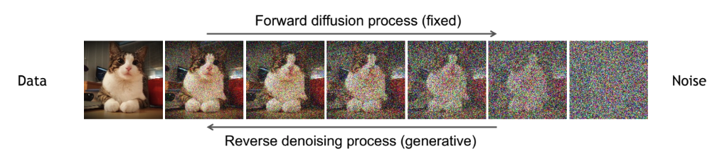
Diffusion models are a powerful class of generative models that learn to create data—such as images—by reversing a gradual noising process. During training, real data is progressively corrupted by adding small amounts of Gaussian noise over many steps until it becomes nearly indistinguishable from pure noise. A neural network is then trained to learn the reverse process: transforming noise back into realistic samples, one step at a time.
Adapted from the CVPR 2023 Tutorial on Diffusion Models by Arash Vahdat.
This approach has enabled state-of-the-art results in image generation, powering tools like DALL·E 2, Imagen, and Stable Diffusion. One of the key advantages of diffusion models lies in their training stability and output quality, especially when compared to earlier generative approaches:
- GANs generate sharp images but rely on adversarial training, which can be unstable and prone to mode collapse.
- VAEs are more stable but often produce blurry outputs due to their reliance on Gaussian assumptions and variational approximations.
- Normalizing Flows provide exact log-likelihoods and stable training but require invertible architectures, which limit model expressiveness.
- Diffusion models avoid adversarial dynamics and use a simple denoising objective. This makes them easier to train and capable of producing highly detailed and diverse samples.
This combination of theoretical simplicity, training robustness, and high-quality outputs has made diffusion models one of the most effective generative modeling techniques in use today.
1.1 Connection to VAEs
Diffusion models may seem very different from VAEs at first glance, but they share a surprising number of structural similarities. Both involve a forward process that adds noise and a reverse process that reconstructs data. And both optimize a form of the ELBO — though with very different interpretations.
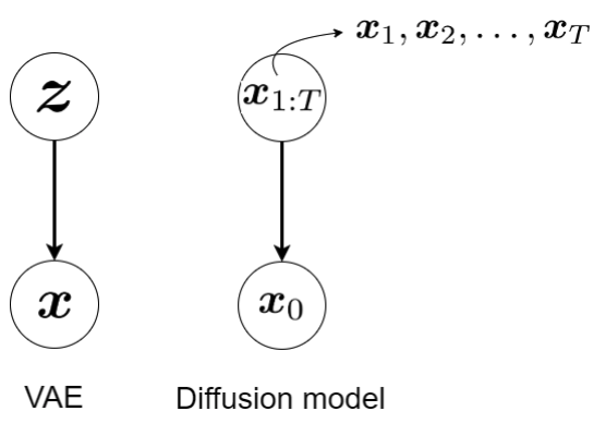
The table below highlights key conceptual parallels:
| Aspect | VAEs | Diffusion Models |
|---|---|---|
| Forward process | Learned encoder \(q_\phi(z \mid x)\) | Fixed noising process \(q(x_t \mid x_{t-1})\) |
| Reverse process | Learned decoder \(p_\theta(x \mid z)\) | Learned denoising model \(p_\theta(x_{t-1} \mid x_t)\) |
| Latent space | Explicit latent variable \(z\) | No explicit latent; \(x_t\) acts as noisy latent |
| Training objective | Maximize ELBO over \(z\) | Maximize ELBO via simplified KL terms and noise prediction |
1.2 Real-World Applications of Diffusion Models
Diffusion models have rapidly moved from research labs to real-world applications. Today, they power many state-of-the-art generative tools:
1.2.1 Text-to-Image
- DALL·E 2 (OpenAI): Generates realistic images from text prompts.
- Imagen (Google): Leverages powerful language encoders for high-fidelity image synthesis.
1.2.2 Text-to-Video
- Make-A-Video (Meta): Extends image models to video generation using textual input.
- Imagen Video (Google): Builds on Imagen to generate coherent video sequences.
1.2.3 Text-to-3D
- DreamFusion (Google): Produces 3D scenes from text by combining diffusion with 3D rendering techniques.
These use cases highlight why diffusion models are considered one of the most promising families of generative models today. To understand how these systems operate, we’ll first explore the mathematical core of diffusion models.
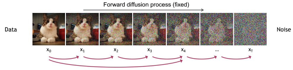
2 Forward Diffusion Process
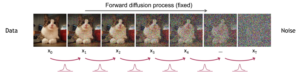
The forward diffusion process gradually turns a data sample (such as an image) into pure noise by adding a little bit of random noise at each step. This process is a Markov chain, meaning each step depends only on the previous one.
2.1 Start with a Data Sample
Begin with a data point \(x_0\), sampled from dataset (such as a real image). The goal is to slowly corrupt \(x_0\) by adding noise over many steps, until it becomes indistinguishable from random Gaussian noise.
We’ll later see that it’s also possible to sample \(x_t\) directly from \(x_0\), without simulating every step.
2.2 Add Noise Recursively
To model the forward diffusion process, we recursively add Gaussian noise at each step. Each step \(q(x_t \mid x_{t-1})\) is defined as a Gaussian distribution, where the mean retains a fraction of the signal from the previous step and the variance controls the amount of noise added.
We define the noise schedule as a sequence of small positive values \(\{ \beta_1, \beta_2, \dots, \beta_T \}\), where \(\beta_t \in (0, 1)\) controls how much noise is injected at step \(t\).
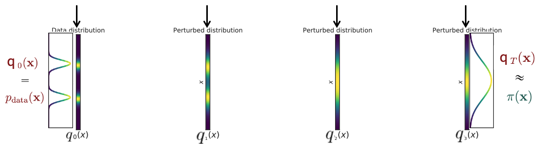
To visualize the effect of the forward process on the entire data distribution (not just individual samples), consider the following:
Adapted from Stanford CS236: Deep Generative Models (Winter 2023).
\[ q(x_t \mid x_{t-1}) = \mathcal{N}(x_t; \sqrt{1 - \beta_t} \, x_{t-1}, \beta_t \, \mathbf{I}) \]
For convenience, we define:
- \(\alpha_t = 1 - \beta_t\) (signal retention at step \(t\))
- \(\bar{\alpha}_t = \prod_{s=1}^{t} \alpha_s\) (cumulative signal retention up to step \(t\))
This lets us express the forward process directly in terms of the original data \(x_0\):
\[ q(x_t \mid x_0) = \mathcal{N}(x_t; \sqrt{\bar{\alpha}_t} \, x_0, (1 - \bar{\alpha}_t) \, \mathbf{I}) \]
At each step, the signal is scaled down by a factor of \(\sqrt{\alpha_t}\), and new Gaussian noise is added with variance \((1 - \alpha_t)\). After many steps, the sample becomes increasingly noisy and approaches an isotropic Gaussian distribution.
Intuition: The signal shrinks gradually while fresh noise is added. Over many steps, the data becomes indistinguishable from pure noise.
Adapted from the CVPR 2023 Tutorial on Diffusion Models by Arash Vahdat.
Choosing small values of \(\beta_t\) ensures that noise is added gradually at each step, allowing the model to retain structure over time. This makes the reverse process easier to learn, as the signal decays smoothly via \(\sqrt{\bar{\alpha}_t}\) rather than being overwhelmed by noise. Large \(\beta_t\) values, on the other hand, can destroy signal too quickly, leading to poor reconstructions.
The choice of \(\beta_t\) at each step—known as the noise schedule—plays a critical role in how effectively the model can learn the reverse denoising process. A well-designed schedule balances signal retention and noise addition, ensuring gradual degradation of structure without overwhelming the data too early. In the next section, we compare common scheduling strategies and their effect on training and image quality.
2.3 Noise Schedules: Linear vs Cosine
The noise schedule determines how much Gaussian noise is added at each step via the sequence \(\{\beta_1, \beta_2, \dots, \beta_T\}\). A well-designed schedule ensures that noise increases gradually—preserving structure early on and enabling the model to learn the reverse process more effectively.
Two commonly used schedules are:
Linear Schedule
In a linear schedule, \(\beta_t\) increases linearly from a small to a larger value. This causes the retained signal \(\bar{\alpha}_t\) to decay rapidly, injecting noise aggressively in early steps. As a result, fine details are lost early, making denoising more difficult.
Cosine Schedule
Cosine schedules are designed to make \(\bar{\alpha}_t\) follow a smooth cosine decay curve. This retains more signal over a longer period, allowing the model to degrade structure more gradually and learn a more stable denoising path.
2.3.1 Visualizing Signal and Noise Tradeoffs
The following plot compares signal preservation and noise growth across the diffusion process for linear and cosine schedules:
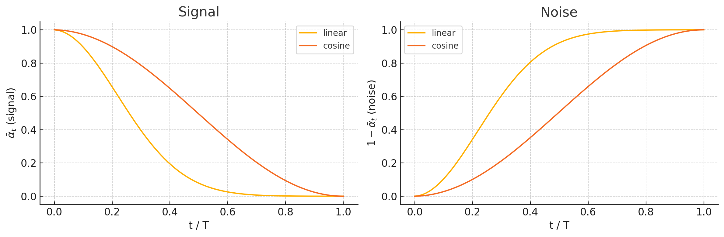
The cosine schedule maintains more signal during early and middle steps, whereas the linear schedule injects noise quickly, causing structure to be lost early in the process.
2.3.2 Visualizing Effects on Images
This plot shows how an image is progressively corrupted under each schedule:
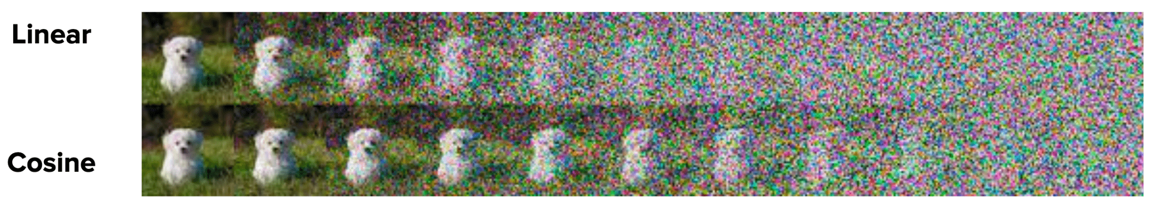
Adapted from Nichol & Dhariwal (2021), “Improved Denoising Diffusion Probabilistic Models”, arXiv:2102.09672.
Cosine schedules preserve details longer, while linear schedules degrade the image more aggressively in fewer steps—highlighting why noise scheduling is critical for downstream generation quality.
2.3.3 Takeaways
- Cosine schedules produce better sample quality by preserving image structure longer.
- Linear schedules are simpler but may hinder training due to early signal loss.
- Most modern diffusion models (e.g., Stable Diffusion, Imagen) prefer cosine schedules for their superior denoising behavior.
- Use a cosine schedule if your goal is to generate high-quality samples or train a stable diffusion model. It preserves structure longer and results in smoother denoising.
- A linear schedule may be acceptable for simple tasks or quick experimentation but can inject noise too aggressively in early steps.
- Always visualize your \(\bar{\alpha}_t\) or signal-to-noise ratio across timesteps to understand how your schedule behaves.
- Many libraries (e.g., Hugging Face diffusers, OpenAI’s improved DDPM repo) implement cosine schedules by default—use these as reliable starting points.
2.4 The Markov Chain
The forward diffusion process forms a Markov chain: each state \(x_t\) depends only on the previous state \(x_{t-1}\). This property enables efficient sampling and simplifies the math behind both training and generation.
The full sequence can be written as:
\[ x_0 \rightarrow x_1 \rightarrow x_2 \rightarrow \cdots \rightarrow x_T \]
The joint probability over all noisy samples given the original data \(x_0\) is:
\[ q(x_{1:T} \mid x_0) = \prod_{t=1}^{T} q(x_t \mid x_{t-1}) \]
This formulation means we can generate the full noise trajectory by repeatedly applying the noise step defined earlier.
Insight: Even though we can sample any \(x_t\) directly from \(x_0\) using a closed-form Gaussian, modeling the full Markov chain is still essential. It forms the foundation for defining the reverse (denoising) process, which we’ll learn next.
2.5 Deriving the Marginal Distribution \(q(x_t \mid x_0)\)
So far, we’ve modeled the full Markov chain step-by-step. But how do we compute \(x_t\) directly from \(x_0\), without simulating each intermediate step?
Let’s see how \(x_t\) accumulates noise from \(x_0\).
For \(t = 1\): \[ x_1 = \sqrt{\alpha_1} x_0 + \sqrt{1 - \alpha_1} \epsilon_1, \qquad \epsilon_1 \sim \mathcal{N}(0, I) \]
For \(t = 2\): \[ x_2 = \sqrt{\alpha_2} x_1 + \sqrt{1 - \alpha_2} \epsilon_2 \] Substitute \(x_1\): \[ x_2 = \sqrt{\alpha_2} \left( \sqrt{\alpha_1} x_0 + \sqrt{1 - \alpha_1} \epsilon_1 \right) + \sqrt{1 - \alpha_2} \epsilon_2 \] \[ = \sqrt{\alpha_2 \alpha_1} x_0 + \sqrt{\alpha_2 (1 - \alpha_1)} \epsilon_1 + \sqrt{1 - \alpha_2} \epsilon_2 \]
For general \(t\), recursively expanding gives: \[ x_t = \sqrt{\bar{\alpha}_t} x_0 + \sum_{i=1}^t \left( \sqrt{ \left( \prod_{j=i+1}^t \alpha_j \right) (1 - \alpha_i) } \, \epsilon_i \right) \] where \(\bar{\alpha}_t = \prod_{i=1}^t \alpha_i\).
Each \(\epsilon_i\) is independent Gaussian noise. The sum of independent Gaussians (each scaled by a constant) is still a Gaussian, with variance equal to the sum of the variances: \[ \text{Total variance} = \sum_{i=1}^t \left( \prod_{j=i+1}^t \alpha_j \right) (1 - \alpha_i) \] This sum simplifies to: \[ 1 - \bar{\alpha}_t \]
This can be proved by induction or by telescoping the sum.
All the little bits of noise added at each step combine into one big Gaussian noise term, with variance \(1 - \bar{\alpha}_t\).
2.6 The Final Marginal Distribution
So, we can sample \(x_t\) directly from \(x_0\) using: \[ x_t = \sqrt{\bar{\alpha}_t} x_0 + \sqrt{1 - \bar{\alpha}_t} \epsilon, \qquad \epsilon \sim \mathcal{N}(0, I) \]
This lets us sample \(x_t\) directly from \(x_0\), without recursively computing all previous steps \(x_1, x_2, \dots, x_{t-1}\).
This means: \[ q(x_t \mid x_0) = \mathcal{N}\left(x_t; \sqrt{\bar{\alpha}_t} x_0, (1 - \bar{\alpha}_t) I\right) \]
As \(t\) increases, \(\bar{\alpha}_t\) shrinks toward zero. Eventually, \(x_t\) becomes pure noise:
\[ x_T \sim \mathcal{N}(0, I) \]
Adapted from the CVPR 2023 Tutorial on Diffusion Models by Arash Vahdat.
2.7 Recap: Forward Diffusion Steps
| Step | Formula | Explanation |
|---|---|---|
| 1 | \(x_0\) | Original data sample |
| 2 | \(q(x_t \mid x_{t-1}) = \mathcal{N}(\sqrt{\alpha_t} x_{t-1}, (1-\alpha_t) I)\) | Add noise at each step |
| 3 | \(x_t = \sqrt{\bar{\alpha}_t} x_0 + \sqrt{1 - \bar{\alpha}_t} \, \epsilon\) | Directly sample \(x_t\) from \(x_0\) using noise \(\epsilon\) |
| 4 | \(q(x_t \mid x_0) = \mathcal{N}(\sqrt{\bar{\alpha}_t} x_0, (1-\bar{\alpha}_t) I)\) | Marginal distribution at step \(t\) |
| 5 | \(x_T \sim \mathcal{N}(0, I)\) | After many steps, pure noise |
2.8 Key Takeaways
- The forward diffusion process is just repeatedly adding noise to your data.
- Thanks to properties of Gaussian noise, you can describe the result as the original data scaled down plus one cumulative chunk of Gaussian noise.
- After enough steps, the data becomes indistinguishable from random noise.
3 Reverse Diffusion Process
Let’s break down the reverse diffusion process step by step. This is the generative phase of diffusion models, where we learn to turn pure noise back into data. For clarity, we’ll use the same notation as in the forward process:
- Forward process: Gradually adds noise to data via \(q(x_t \mid x_{t-1})\)
- Reverse process: Gradually removes noise via \(p_\theta(x_{t-1} \mid x_t)\), learned by a neural network
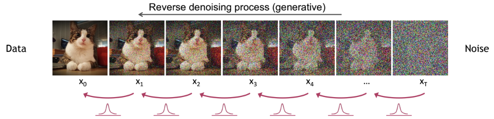
Adapted from the CVPR 2023 Tutorial on Diffusion Models by Arash Vahdat.
The Goal of the Reverse Process
Objective: Given a noisy sample \(x_t\), we want to estimate the conditional distribution \(q(x_{t-1} \mid x_t)\). However, this is intractable because it would require knowing the true data distribution.
Instead, we train a neural network to approximate it: \[ p_\theta(x_{t-1} \mid x_t) = \mathcal{N}(x_{t-1}; \mu_\theta(x_t, t), \Sigma_\theta(x_t, t)) \]
Here, \(\mu_\theta(x_t, t)\) is the predicted mean and \(\Sigma_\theta(x_t, t)\) is the predicted covariance (often diagonal) of the reverse Gaussian distribution. In many implementations, the variance \(\Sigma_\theta(x_t, t)\) is either fixed or parameterized separately, so the model focuses on learning the mean \(\mu_\theta(x_t, t)\) during training.
In practice, many diffusion models do not directly predict \(\mu_\theta\) or \(x_0\), but instead predict the noise \(\epsilon\) added in the forward process. This makes the objective simpler and more effective, as we’ll see in the next section.
Key Insight from the Forward Process
If the noise added in the forward process is small (i.e., \(\beta_t \ll 1\)), then the reverse conditional \(q(x_{t-1} \mid x_t)\) is also Gaussian: \[ q(x_{t-1} \mid x_t) \approx \mathcal{N}(x_{t-1}; \tilde{\mu}_t(x_t), \tilde{\beta}_t I) \]
This approximation works because the forward process adds Gaussian noise in small increments at each step. The Markov chain formed by these small Gaussian transitions ensures that local conditionals (like \(q(x_{t-1} \mid x_t)\)) remain Gaussian under mild assumptions.
- \(\alpha_t\): Variance-preserving noise coefficient at step \(t\)
- \(\bar{\alpha}_t\): Cumulative product of \(\alpha_t\), i.e., \(\bar{\alpha}_t = \prod_{s=1}^t \alpha_s\)
- \(\beta_t\): Variance of the noise added at step \(t\), typically \(\beta_t = 1 - \alpha_t\)
- \(x_0\): Original clean data sample (e.g., image)
- \(x_t\): Noisy version of \(x_0\) at timestep \(t\)
- \(\epsilon\): Standard Gaussian noise sampled from \(\mathcal{N}(0, I)\)
- \(\tilde{\mu}_t\): Mean of the reverse process distribution at time \(t\)
- \(\tilde{\beta}_t\): Variance of the reverse process distribution at time \(t\)
3.1 Deriving \(q(x_{t-1} \mid x_t, x_0)\) Using Bayes’ Rule
We can’t directly evaluate \(q(x_{t-1} \mid x_t)\), but we can derive the posterior \(q(x_{t-1} \mid x_t, x_0)\) using Bayes’ rule:
\[ q(x_{t-1} \mid x_t, x_0) = \frac{q(x_t \mid x_{t-1}, x_0) \cdot q(x_{t-1} \mid x_0)}{q(x_t \mid x_0)} \]
From the forward process, we know:
- \(q(x_t \mid x_{t-1}) = \mathcal{N}(x_t; \sqrt{\alpha_t} x_{t-1},\, \beta_t I)\)
- \(q(x_{t-1} \mid x_0) = \mathcal{N}(x_{t-1}; \sqrt{\bar{\alpha}_{t-1}} x_0,\, (1 - \bar{\alpha}_{t-1}) I)\)
- \(q(x_t \mid x_0) = \mathcal{N}(x_t; \sqrt{\bar{\alpha}_t} x_0,\, (1 - \bar{\alpha}_t) I)\)
To derive a usable form of the posterior, we substitute the Gaussian densities into Bayes’ rule. The multivariate normal density is:
\[ \mathcal{N}(x \mid \mu, \Sigma) \propto \exp\left( -\frac{1}{2}(x - \mu)^T \Sigma^{-1} (x - \mu) \right) \]
Since all covariances here are multiples of the identity matrix, \(\Sigma = \sigma^2 I\), the formula simplifies to:
\[ \mathcal{N}(x \mid \mu, \sigma^2 I) \propto \exp\left( -\frac{1}{2\sigma^2} \|x - \mu\|^2 \right) \]
The expression \(\|x - \mu\|^2\) is the squared distance between two vectors. In 1D, it’s just \((x - \mu)^2\), but in higher dimensions, it becomes:
\[ \|x - \mu\|^2 = \sum_{i=1}^d (x_i - \mu_i)^2 \]
This term appears in the exponent of the Gaussian and represents how far the sample is from the center (mean), scaled by the variance.
Applying this to the forward process terms:
- \(q(x_t \mid x_{t-1}) \propto \exp\left( -\frac{1}{2\beta_t} \| x_t - \sqrt{\alpha_t} x_{t-1} \|^2 \right)\)
- \(q(x_{t-1} \mid x_0) \propto \exp\left( -\frac{1}{2(1 - \bar{\alpha}_{t-1})} \| x_{t-1} - \sqrt{\bar{\alpha}_{t-1}} x_0 \|^2 \right)\)
We can ignore \(q(x_t \mid x_0)\) in the denominator, since it is independent of \(x_{t-1}\) and will be absorbed into a proportionality constant.
Putting these together:
\[ q(x_{t-1} \mid x_t, x_0) \propto \exp\left( -\frac{1}{2} \left[ \frac{ \|x_t - \sqrt{\alpha_t} x_{t-1} \|^2 }{\beta_t} + \frac{ \| x_{t-1} - \sqrt{\bar{\alpha}_{t-1}} x_0 \|^2 }{1 - \bar{\alpha}_{t-1}} \right] \right) \]
When we multiply two Gaussian distributions over the same variable, the result is also a Gaussian.
Here, we are multiplying two Gaussians in \(x_{t-1}\):
- One centered at \(\sqrt{\alpha_t} x_t\)
- One centered at \(\sqrt{\bar{\alpha}_{t-1}} x_0\)
The product is another Gaussian in \(x_{t-1}\), with a new mean that is a weighted average of both.
We’ll derive this explicitly by completing the square in the exponent.
Although we won’t use this posterior directly during sampling, this closed-form expression is essential for defining the ELBO used in training. It gives us a precise target that the reverse model attempts to approximate.
We now complete the square to put the expression into standard Gaussian form.
3.2 Complete the square
We complete the square by rewriting the quadratic expression in a way that matches the standard form of a Gaussian. This lets us rewrite the posterior \(q(x_{t-1} \mid x_t, x_0)\) in standard Gaussian form by identifying its mean and variance.
\[ a x^2 - 2 b x = a \left( x - \frac{b}{a} \right)^2 - \frac{b^2}{a} \]
From earlier, we arrived at this expression for the exponent of the posterior:
\[
-\frac{1}{2} \left[
\frac{(x_t - \sqrt{\alpha_t} \, x_{t-1})^2}{\beta_t} +
\frac{(x_{t-1} - \sqrt{\bar{\alpha}_{t-1}} \, x_0)^2}{1 - \bar{\alpha}_{t-1}}
\right]
\]
We expand both terms:
First term:
\[
\frac{(x_t - \sqrt{\alpha_t} \, x_{t-1})^2}{\beta_t}
= \frac{x_t^2 - 2 \sqrt{\alpha_t} \, x_t x_{t-1} + \alpha_t x_{t-1}^2}{\beta_t}
\]
Second term:
\[
\frac{(x_{t-1} - \sqrt{\bar{\alpha}_{t-1}} \, x_0)^2}{1 - \bar{\alpha}_{t-1}}
= \frac{x_{t-1}^2 - 2 \sqrt{\bar{\alpha}_{t-1}} \, x_{t-1} x_0 + \bar{\alpha}_{t-1} x_0^2}{1 - \bar{\alpha}_{t-1}}
\]
Group like terms
Now we collect all the terms involving \(x_{t-1}\):
Coefficient of \(x_{t-1}^2\):
\[
a = \frac{\alpha_t}{\beta_t} + \frac{1}{1 - \bar{\alpha}_{t-1}}
\]
Coefficient of \(x_{t-1}\) (the full linear term):
\[
-2 \left(
\frac{ \sqrt{\alpha_t} \, x_t }{ \beta_t } + \frac{ \sqrt{\bar{\alpha}_{t-1}} \, x_0 }{ 1 - \bar{\alpha}_{t-1} }
\right)
\]
So we define:
\[
b = \frac{ \sqrt{\alpha_t} \, x_t }{ \beta_t } + \frac{ \sqrt{\bar{\alpha}_{t-1}} \, x_0 }{ 1 - \bar{\alpha}_{t-1} }
\]
Remaining terms (like \(x_t^2\) and \(x_0^2\)) are independent of \(x_{t-1}\) and can be absorbed into a constant.
We are modeling the conditional distribution \(q(x_{t-1} \mid x_t, x_0)\), which means both \(x_t\) and \(x_0\) are known and fixed. So any expression involving only \(x_t\) or \(x_0\) behaves like a constant and does not influence the shape of the Gaussian over \(x_{t-1}\).
The exponent now has the form:
\[
-\frac{1}{2} \left( a x_{t-1}^2 - 2 b x_{t-1} \right) + \text{(constants)}
\]
Apply the identity
Using the identity: \[ a x^2 - 2 b x = a \left( x - \frac{b}{a} \right)^2 - \frac{b^2}{a} \]
we rewrite the exponent: \[ -\frac{1}{2} \left( a x_{t-1}^2 - 2 b x_{t-1} \right) = -\frac{1}{2} \left[ a \left( x_{t-1} - \frac{b}{a} \right)^2 - \frac{b^2}{a} \right] \]
We drop the constant term \(\frac{b^2}{a}\) under proportionality. This transforms the exponent into the Gaussian form: \[ q(x_{t-1} \mid x_t, x_0) \propto \exp\left( - \frac{1}{2 \tilde{\beta}_t} \| x_{t-1} - \tilde{\mu}_t \|^2 \right) \]
The standard Gaussian is written as: \[ \mathcal{N}(x \mid \mu, \sigma^2 I) \propto \exp\left( - \frac{1}{2\sigma^2} \| x - \mu \|^2 \right) \]
So in our case:
- \(\tilde{\mu}_t = \frac{b}{a}\) is the mean
- \(\tilde{\beta}_t = \frac{1}{a}\) is the variance
We keep the notation \(\tilde{\beta}_t\) instead of \(\sigma^2\) because it connects directly to the noise schedule (\(\beta_t\), \(\bar{\alpha}_t\)) used in the diffusion model. This helps tie everything back to how the forward and reverse processes relate.
Final expressions
Now we can directly read off the expressions for the mean and variance from the completed square.
We had: \[ a = \frac{\alpha_t}{\beta_t} + \frac{1}{1 - \bar{\alpha}_{t-1}}, \quad b = \frac{\sqrt{\alpha_t} \, x_t}{\beta_t} + \frac{\sqrt{\bar{\alpha}_{t-1}} \, x_0}{1 - \bar{\alpha}_{t-1}} \]
From the identity: \[ q(x_{t-1} \mid x_t, x_0) \propto \exp\left( - \frac{1}{2 \tilde{\beta}_t} \| x_{t-1} - \tilde{\mu}_t \|^2 \right) \]
we identify: - \(\tilde{\mu}_t = \frac{b}{a}\), - \(\tilde{\beta}_t = \frac{1}{a}\)
Let’s compute these explicitly:
Mean: \[ \tilde{\mu}_t = \frac{b}{a} = \frac{ \sqrt{\alpha_t}(1 - \bar{\alpha}_{t-1}) x_t + \sqrt{\bar{\alpha}_{t-1}} \beta_t x_0 }{ 1 - \bar{\alpha}_t } \]
Variance: \[ \tilde{\beta}_t = \frac{1}{a} = \frac{1 - \bar{\alpha}_{t-1}}{1 - \bar{\alpha}_t} \cdot \beta_t \]
So the final expression for the posterior becomes: \[ q(x_{t-1} \mid x_t, x_0) = \mathcal{N}(x_{t-1};\, \tilde{\mu}_t,\, \tilde{\beta}_t I) \]
3.3 Parameterizing the Reverse Process
During training, we can compute the posterior exactly because \(x_0\) is known. But at sampling time, we don’t have access to \(x_0\), so we must express everything in terms of the current noisy sample \(x_t\) and the model’s prediction of noise \(\epsilon\).
We start from the forward noising equation:
\[ x_t = \sqrt{\bar{\alpha}_t} \, x_0 + \sqrt{1 - \bar{\alpha}_t} \, \epsilon \]
This expresses how noise is added to the clean image \(x_0\) to produce the noisy observation \(x_t\).
We rearrange this to solve for \(x_0\) in terms of \(x_t\) and \(\epsilon\):
\[ x_0 = \frac{x_t - \sqrt{1 - \bar{\alpha}_t} \, \epsilon}{\sqrt{\bar{\alpha}_t}} \]
Now we substitute this into the posterior mean expression \(\tilde{\mu}_t\), which originally depended on \(x_0\):
\[ \tilde{\mu}_t = \frac{ \sqrt{\alpha_t}(1 - \bar{\alpha}_{t-1}) x_t + \sqrt{\bar{\alpha}_{t-1}} \beta_t x_0 }{ 1 - \bar{\alpha}_t } \]
Substituting \(x_0\) into this gives:
\[ \tilde{\mu}_t = \frac{1}{\sqrt{\alpha_t}} \left( x_t - \frac{\beta_t}{\sqrt{1 - \bar{\alpha}_t}} \, \epsilon \right) \]
This allows us to compute the mean of the reverse process using only \(x_t\), \(\epsilon\), and known scalars from the noise schedule.
- \(\epsilon\) is the noise that was added to \(x_0\) to get \(x_t\)
- At test time, we use the model’s prediction \(\epsilon_\theta(x_t, t)\) in its place
3.4 Recap: Reverse Diffusion Steps
| Step | Formula | Explanation |
|---|---|---|
| 1 | \(q(x_{t-1} \mid x_t, x_0)\) | True posterior used during training (when \(x_0\) is known) |
| 2 | \(\tilde{\mu}_t = \dfrac{1}{\sqrt{\alpha_t}} \left( x_t - \dfrac{\beta_t}{\sqrt{1 - \bar{\alpha}_t}} \, \epsilon \right)\) | Posterior mean rewritten using \(x_t\) and noise |
| 3 | \(\epsilon \approx \epsilon_\theta(x_t, t)\) | At test time, model predicts the noise |
| 4 | \(p_\theta(x_{t-1} \mid x_t) = \mathcal{N}(\tilde{\mu}_t, \tilde{\beta}_t I)\) | Reverse step sampled from model’s predicted mean and fixed variance |
3.5 Key Takeaways
- The reverse diffusion process defines a learned Markov chain that gradually removes noise from the input.
- Although we can’t compute the true reverse distribution \(q(x_{t-1} \mid x_t)\), we derive a tractable Gaussian approximation using Bayes’ rule.
- The reverse mean depends on both \(x_t\) and the original data \(x_0\), but at test time we use the model’s prediction of noise \(\epsilon_\theta(x_t, t)\) to estimate \(x_0\).
- The reverse steps preserve a Gaussian structure, enabling efficient sampling using the predicted mean \(\mu_\theta(x_t, t)\) and fixed variance \(\Sigma_\theta(x_t, t)\).
4 Training: Understanding the ELBO
What is the Goal? The ultimate goal in diffusion models is to train the neural network so that it can reverse the noising process. In other words, we want the network to learn how to turn random noise back into realistic data (like images). But how do we actually train the network? We need a loss function—a way to measure how good or bad the network’s predictions are, so we can improve it.
4.1 What is the ELBO?
The ELBO is a lower bound on the log-likelihood of the data. Maximizing the ELBO is equivalent to maximizing the likelihood that the model can generate the training data. For diffusion models, the ELBO ensures that the reverse process (denoising) aligns with the forward process (noising).
Note: For a foundational introduction to the ELBO and its role in generative models, see my Variational Autoencoder (VAE) post at changezakram.github.io/Deep-Generative-Models/vae.html.
4.2 Deriving the ELBO for Diffusion Models
Goal:
We want to maximize the log-likelihood of the data:
\[ \log p_\theta(x_0) \]
where \(x_0\) is a clean data sample (e.g., an image).
Problem:
Computing \(\log p_\theta(x_0)\) directly is intractable because it involves integrating over all possible noisy intermediate states \(x_{1:T}\).
Solution:
Use Jensen’s Inequality to derive a lower bound (the ELBO) that we can optimize instead.
4.3 Full Derivation (Step-by-Step)
Step 1: Start with the log-likelihood
\[ \log p_\theta(x_0) = \log \int p_\theta(x_{0:T}) \, dx_{1:T} \]
Step 2: Introduce the forward process \(q(x_{1:T} \mid x_0)\)
Multiply and divide by the fixed forward process:
\[ \log p_\theta(x_0) = \log \int \frac{p_\theta(x_{0:T})}{q(x_{1:T} \mid x_0)} q(x_{1:T} \mid x_0) \, dx_{1:T} \]
Step 3: Rewrite as an expectation
\[ \log p_\theta(x_0) = \log \mathbb{E}_{q(x_{1:T} \mid x_0)} \left[ \frac{p_\theta(x_{0:T})}{q(x_{1:T} \mid x_0)} \right] \]
Step 4: Apply Jensen’s Inequality
\[ \log p_\theta(x_0) \geq \mathbb{E}_{q(x_{1:T} \mid x_0)} \left[ \log \frac{p_\theta(x_{0:T})}{q(x_{1:T} \mid x_0)} \right] \]
Step 5: Expand \(p_\theta(x_{0:T})\) and \(q(x_{1:T} \mid x_0)\)
The reverse (generative) process is:
\[ p_\theta(x_{0:T}) = p(x_T) \cdot \prod_{t=1}^T p_\theta(x_{t-1} \mid x_t) \]
The forward (noising) process is:
\[ q(x_{1:T} \mid x_0) = \prod_{t=1}^T q(x_t \mid x_{t-1}) \]
Substitute both into the ELBO:
\[ \text{ELBO} = \mathbb{E}_{q(x_{1:T} \mid x_0)} \left[ \log \left( \frac{p(x_T) \cdot \prod_{t=1}^T p_\theta(x_{t-1} \mid x_t)} {\prod_{t=1}^T q(x_t \mid x_{t-1})} \right) \right] \]
Split the logarithm:
\[ \text{ELBO} = \mathbb{E}_{q(x_{1:T} \mid x_0)} \left[ \log p(x_T) + \sum_{t=1}^T \log p_\theta(x_{t-1} \mid x_t) - \sum_{t=1}^T \log q(x_t \mid x_{t-1}) \right] \]
Group the terms:
\[ \text{ELBO} = \mathbb{E}_{q(x_{1:T} \mid x_0)} \left[ \log p(x_T) + \sum_{t=1}^T \log \frac{p_\theta(x_{t-1} \mid x_t)}{q(x_t \mid x_{t-1})} \right] \]
Step 6: Decompose the ELBO
We now break down the Evidence Lower Bound (ELBO) into three interpretable components:
- The prior loss — how well the final noisy sample matches the prior
- The denoising KL terms — how well the model learns to denoise at each timestep
- The reconstruction loss — how well the model recovers the original input
ELBO Expression from Previous Step
\[ = \mathbb{E}_{q(x_{1:T} \mid x_0)} \left[ \log p(x_T) + \sum_{t=1}^T \log \frac{p_\theta(x_{t-1} \mid x_t)}{q(x_t \mid x_{t-1})} \right] \]
Isolating the Reconstruction Term
The case for \(t = 1\) is special: it’s the step where the model tries to reconstruct \(x_0\) from \(x_1\). So we isolate it from the rest of the trajectory-based KL terms.
\[ = \mathbb{E}_{q(x_{1:T} \mid x_0)} \left[ \log p(x_T) + \sum_{t=2}^T \log \frac{p_\theta(x_{t-1} \mid x_t)}{q(x_t \mid x_{t-1})} + \log \frac{p_\theta(x_0 \mid x_1)}{q(x_1 \mid x_0)} \right] \]
Rewriting Using the Known Forward Process
The forward process gives us a complete description of how noise is added to data. Because of this, we can calculate the exact probability of earlier steps given later ones. In particular, since both \(x_t\) and \(x_0\) are known during training, we can compute the true backward distribution \(q(x_{t-1} \mid x_t, x_0)\). This lets us directly compare it to the model’s learned reverse process \(p_\theta(x_{t-1} \mid x_t)\).
This gives:
\[ = \mathbb{E}_{q(x_{1:T} \mid x_0)} \left[ \log p(x_T) + \sum_{t=2}^T \log \frac{p_\theta(x_{t-1} \mid x_t)}{q(x_{t-1} \mid x_t, x_0)} + \log p_\theta(x_0 \mid x_1) - \log q(x_1 \mid x_0) \right] \]
The last term, \(\log q(x_1 \mid x_0)\), comes from the known forward process and does not depend on the model parameters. Since it stays constant during training, we drop it from the objective and retain the remaining three terms.
The first two log-ratios can now be rewritten as KL divergences, and the third term becomes a standard reconstruction loss.
Rewriting the First Term as a KL Divergence
We begin with the first term from the ELBO expression:
\[ \mathbb{E}_{q(x_{1:T} \mid x_0)} \left[ \log p(x_T) \right] \]
Since this expectation only involves \(x_T\), we can simplify it as:
\[ \mathbb{E}_{q(x_T \mid x_0)} \left[ \log p(x_T) \right] \]
Now recall the definition of KL divergence between two distributions \(q(x)\) and \(p(x)\):
\[ D_{\text{KL}}(q(x) \,\|\, p(x)) = \mathbb{E}_{q(x)} \left[ \log \frac{q(x)}{p(x)} \right] = \mathbb{E}_{q(x)} [\log q(x)] - \mathbb{E}_{q(x)} [\log p(x)] \]
Rearranging this gives:
\[ \mathbb{E}_{q(x)} [\log p(x)] = -D_{\text{KL}}(q(x) \,\|\, p(x)) + \mathbb{E}_{q(x)} [\log q(x)] = -D_{\text{KL}}(q(x) \,\|\, p(x)) + \mathbb{H}[q(x)] \]
Applying this identity to \(q(x_T \mid x_0)\) — which is analytically tractable due to the known forward process — and the prior \(p(x_T)\):
\[ \mathbb{E}_{q(x_T \mid x_0)} [\log p(x_T)] = -D_{\text{KL}}(q(x_T \mid x_0) \,\|\, p(x_T)) + \mathbb{H}[q(x_T \mid x_0)] \]
Since \(q(x_T \mid x_0)\) is part of the fixed forward process, its entropy \(\mathbb{H}[q(x_T \mid x_0)]\) is independent of model parameters and can be ignored during training. So we drop it:
\[ \mathbb{E}_{q(x_T \mid x_0)} [\log p(x_T)] \approx -D_{\text{KL}}(q(x_T \mid x_0) \parallel p(x_T)) \quad \text{(ignoring constant entropy term)} \]
This shows that the first term in the ELBO corresponds to \(D_{\text{KL}}(q(x_T \mid x_0) \,\|\, p(x_T))\), comparing the forward process at time \(T\) to the model’s prior.
Rewriting the Second Terms as KL Divergences
Next, we consider the sum of log-ratio terms from the ELBO expression:
\[ \sum_{t=2}^T \mathbb{E}_q \left[ \log \frac{p_\theta(x_{t-1} \mid x_t)}{q(x_{t-1} \mid x_t, x_0)} \right] \]
This expression compares two distributions:
- \(p_\theta(x_{t-1} \mid x_t)\): the model’s learned reverse (denoising) process
- \(q(x_{t-1} \mid x_t, x_0)\): the true posterior over \(x_{t-1}\) given \(x_t\) and the original data \(x_0\)
(this is computable in closed-form since the forward process is known)
Now recall the definition of KL divergence:
\[ D_{\text{KL}}(q(x) \,\|\, p(x)) = \mathbb{E}_{q(x)} \left[ \log \frac{q(x)}{p(x)} \right] \]
If we flip the log-ratio, we get:
\[ \mathbb{E}_{q(x)} \left[ \log \frac{p(x)}{q(x)} \right] = - D_{\text{KL}}(q(x) \,\|\, p(x)) \]
So each log term becomes the negative KL divergence:
\[ \mathbb{E}_q \left[ \log \frac{p_\theta(x_{t-1} \mid x_t)}{q(x_{t-1} \mid x_t, x_0)} \right] = - D_{\text{KL}}(q(x_{t-1} \mid x_t, x_0) \,\|\, p_\theta(x_{t-1} \mid x_t)) \]
Applying this for every timestep from \(t = 2\) to \(T\), we get:
\[ \sum_{t=2}^T \mathbb{E}_q \left[ \log \frac{p_\theta(x_{t-1} \mid x_t)}{q(x_{t-1} \mid x_t, x_0)} \right] = - \sum_{t=2}^T D_{\text{KL}}(q(x_{t-1} \mid x_t, x_0) \,\|\, p_\theta(x_{t-1} \mid x_t)) \]
This shows that the middle terms in the ELBO can be rewritten as a sum of KL divergences between the true posterior and the model’s learned reverse process at each timestep.
Rewriting the Third Term as a Reconstruction Loss
The last part of the ELBO expression is:
\[ \mathbb{E}_q \left[ \log p_\theta(x_0 \mid x_1) \right] \]
This term does not involve any KL divergence — it directly corresponds to the model’s attempt to reconstruct the original input \(x_0\) from \(x_1\).
- \(x_1\) is a slightly noisy version of \(x_0\) (after one step of the forward process).
- \(p_\theta(x_0 \mid x_1)\) is the model’s decoder — it tries to map the noisy input \(x_1\) back to the clean data \(x_0\).
During training, this term is treated as a standard log-likelihood loss. Since we want to maximize the ELBO, we want to maximize this log-probability — which is equivalent to minimizing the negative log-likelihood:
\[ - \log p_\theta(x_0 \mid x_1) \]
This is why the reconstruction term appears with a positive sign in the loss (as a value we minimize), but a negative sign inside the ELBO.
This is referred to as the reconstruction loss in diffusion models.
If \(p_\theta(x_0 \mid x_1)\) is modeled as a Gaussian, this term becomes a mean squared error between the predicted and true \(x_0\) values.
ELBO vs. Loss
We write the ELBO as:
\[ \text{ELBO} = \underbrace{- D_{\text{KL}}(q(x_T \mid x_0) \parallel p(x_T))}_{\mathcal{L}_T} \quad \underbrace{- \sum_{t=2}^T D_{\text{KL}}(q(x_{t-1} \mid x_t, x_0) \parallel p_\theta(x_{t-1} \mid x_t))}_{\mathcal{L}_{1:T-1}} \quad \underbrace{+ \mathbb{E}_q \left[ \log p_\theta(x_0 \mid x_1) \right]}_{\mathcal{L}_0} \]
Since we minimize loss instead of maximizing ELBO, we flip the sign.
We write the loss as:
\[ \text{Loss} = \underbrace{+ D_{\text{KL}}(q(x_T \mid x_0) \parallel p(x_T))}_{\mathcal{L}_T} \quad \underbrace{+ \sum_{t=2}^T D_{\text{KL}}(q(x_{t-1} \mid x_t, x_0) \parallel p_\theta(x_{t-1} \mid x_t))}_{\mathcal{L}_{1:T-1}} \quad \underbrace{- \mathbb{E}_q \left[ \log p_\theta(x_0 \mid x_1) \right]}_{\mathcal{L}_0} \]
4.4 Interpreting Each Term in the ELBO
Reconstruction Loss (\(\mathcal{L}_0\))
- Encourages the model to reconstruct \(x_0\) from the first noisy sample \(x_1\)
- Comes from the log-probability term \(\log p_\theta(x_0 \mid x_1)\)
- Treated as a negative log-likelihood (e.g., MSE if modeled as Gaussian)
Prior Matching Loss (\(\mathcal{L}_T\))
- Penalizes mismatch between the final noisy sample \(x_T\) and the prior \(p(x_T)\)
- Comes from the KL divergence \(D_{\text{KL}}(q(x_T \mid x_0) \parallel p(x_T))\)
- Ensures the generative process starts from pure noise
Denoising KL Terms (\(\mathcal{L}_{1:T-1}\))
- Encourage the model to learn the correct reverse step at each \(t = 2\) to \(T\)
- Each term compares \(q(x_{t-1} \mid x_t, x_0)\) to the learned \(p_\theta(x_{t-1} \mid x_t)\)
- Drives step-by-step denoising behavior
The ELBO gives us a principled objective that encourages the learned reverse process to match the true posterior. In practice, however, the KL terms can be simplified when we assume Gaussian forward and reverse processes.
This lets us rewrite the training objective in terms of the model’s ability to predict the noise \(\epsilon\) that was added during the forward process.
This lets us rewrite the training objective in terms of the model’s ability to predict the noise \(\epsilon\) that was added during the forward process.
4.5 The core loss used in DDPM training
When all forward and reverse steps in the diffusion process are modeled as Gaussians, the KL terms in the ELBO can be simplified significantly.
For example, the KL divergence between the true posterior \(q(x_{t-1} \mid x_t, x_0)\) and the model’s reverse process \(p_\theta(x_{t-1} \mid x_t)\) becomes:
\[ D_{\text{KL}}\left( q(x_{t-1} \mid x_t, x_0) \;\|\; p_\theta(x_{t-1} \mid x_t) \right) \]
Since both distributions are Gaussian, this KL has a closed-form expression. If we fix the variances and only match the means, minimizing the KL reduces to a squared error loss between the true noise \(\epsilon\) and the model’s prediction \(\epsilon_\theta\).
To approximate the ELBO in practice, DDPM uses a simplified MSE loss between the predicted and true noise:
\[ \mathcal{L}_{\text{simple}} = \mathbb{E}_{x_0, t, \epsilon} \left[ \left\| \epsilon - \epsilon_\theta(x_t, t) \right\|^2 \right] \]
In the forward process, the noisy sample \(x_t\) is generated from \(x_0\) by adding scaled Gaussian noise \(\epsilon\):
\[ x_t = \sqrt{\bar{\alpha}_t} \, x_0 + \sqrt{1 - \bar{\alpha}_t} \, \epsilon \]
The network input originally is \(x_t\), but now we explicitly substitute its definition:
\[ \epsilon_\theta(x_t, t) \quad \Rightarrow \quad \epsilon_\theta\left( \sqrt{\bar{\alpha}_t} \, x_0 + \sqrt{1 - \bar{\alpha}_t} \, \epsilon, \, t \right) \]
We now substitute this new expression into the full loss:
\[ \mathcal{L}_{\text{simple}} = \mathbb{E}_{x_0, t, \epsilon} \left[ \left\| \epsilon - \epsilon_\theta\left( \sqrt{\bar{\alpha}_t} \, x_0 + \sqrt{1 - \bar{\alpha}_t} \, \epsilon, \, t \right) \right\|^2 \right] \]
This is the fully expanded form of the DDPM loss used during training.
- The model receives a noisy input \(x_t\) that is synthesized from \(x_0\) and \(\epsilon\)
- It tries to predict the exact noise \(\epsilon\) that was added
- The loss compares the true noise to the predicted noise, and minimizes their difference using squared error
Even though we end up training with a simplified MSE loss in DDPM, deriving the full ELBO helps us understand what the model is truly learning — and why the simplification works.
- The ELBO gives us a principled, variational objective
- It tells us that training involves matching noise distributions and reconstructing data step-by-step
- The simplified DDPM loss is an approximation of the denoising KL terms (\(\mathcal{L}_{1:T-1}\))
- Other terms (like \(\mathcal{L}_T\) and \(\mathcal{L}_0\)) are often treated as constants or dropped for efficiency
- Many advanced diffusion models return to the ELBO to add back or rethink these terms
So the ELBO is like the blueprint — and the DDPM loss is an optimized shortcut that works because we understand the full path.
4.6 The Noise Prediction Network
Now that we’ve arrived at the simplified training loss used in DDPM, let’s understand what the model is actually learning.
4.6.1 What the Network Learns
- During training, we know the true noise \(\epsilon\) used to generate the noisy sample \(x_t\) from \(x_0\)
- The network \(\epsilon_\theta(x_t, t)\) is trained to predict this noise
- Once trained, the model can use this prediction to “undo” the noise and reconstruct \(x_0\) at test time
4.6.2 Why Predicting Noise Works
Recall the forward process:
\[ x_t = \sqrt{\bar{\alpha}_t} x_0 + \sqrt{1 - \bar{\alpha}_t} \, \epsilon \]
Rearranging this gives an estimate of the original (clean) image:
\[ x_0 = \frac{1}{\sqrt{\bar{\alpha}_t}} \left( x_t - \sqrt{1 - \bar{\alpha}_t} \, \epsilon \right) \]
This is exactly why the DDPM training objective minimizes
\[
\left\| \epsilon - \epsilon_\theta(x_t, t) \right\|^2
\]
— because if we can predict the noise, we can recover the clean image \(x_0\).
This denoised estimate is also used during sampling to compute the mean of the reverse distribution \(q(x_{t-1} \mid x_t, x_0)\) — which is key to reversing the diffusion process one step at a time.
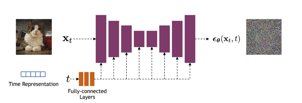
5 U-Net Architecture for Denoising
The network \(\epsilon_\theta(x_t, t)\) is typically implemented as a U-Net, which takes:
- A noisy image \(x_t\)
- A timestep \(t\), encoded using sinusoidal or learned embeddings
It outputs the predicted noise \(\epsilon\), allowing the model to reverse the diffusion process.
The U-Net architecture is particularly effective in diffusion models because it preserves the spatial resolution of the input throughout the network. Unlike VAEs, which compress the input into a lower-dimensional latent space, the U-Net uses skip connections to pass fine-grained information directly from downsampling to upsampling layers. This helps preserve image detail and texture throughout the denoising process.
5.1 Key components of the U-Net used in diffusion models:
- The input is a noisy image (e.g., shape \(64 \times 64 \times 3\)) that we wish to denoise.
- A second input provides the noise variance (or timestep), passed through a sinusoidal embedding function.
- The time embedding is upsampled and concatenated with the noisy image along the channel dimension.
- The combined input is passed through:
- A downsampling path composed of
DownBlocks, which increase the number of channels while reducing spatial dimensions. - Residual blocks at the bottleneck that help learn deeper representations.
- An upsampling path composed of
UpBlocks, which mirror the downsampling layers. - Skip connections between corresponding down and up blocks to preserve spatial detail.
- A downsampling path composed of
- The output is produced by a final \(1 \times 1\) convolutional layer initialized to zeros.
This structure allows the model to iteratively refine and denoise its estimate of the clean image across reverse steps.
Adapted from Stanford CS236: Deep Generative Models (Winter 2023).
5.2 Takeaways
- The ELBO provides a tractable lower bound on the data likelihood \(\log p_\theta(x_0)\), and serves as the theoretical training objective.
- It decomposes into loss terms that align the learned reverse process with the fixed forward noising process, step by step.
- In practice (as in DDPM), training is simplified to minimizing the mean squared error between the true noise \(\epsilon\) and the predicted noise \(\epsilon_\theta(x_t, t)\).
6 Training and Sampling Algorithms (DDPM)
6.1 Algorithm: Training (DDPM)
Steps: - Sample a data point: \(x_0 \sim q(x_0)\)
- Choose a timestep: \(t \sim \text{Uniform}(\{1, \dots, T\})\)
- Sample noise: \(\epsilon \sim \mathcal{N}(0, I)\)
- Take a gradient step to minimize loss
The training loss is:
\[ \mathcal{L}_{\text{simple}} = \mathbb{E}_{x_0, t, \epsilon} \left[ \left\| \epsilon - \epsilon_\theta\left( \sqrt{\bar{\alpha}_t} x_0 + \sqrt{1 - \bar{\alpha}_t} \, \epsilon, t \right) \right\|^2 \right] \]
Explanation
- Sample a real data point \(x_0\)
- Corrupt it to get \(x_t\) using the forward noising process
- Train \(\epsilon_\theta\) to predict the added noise \(\epsilon\)
- Optimize using mean squared error between predicted and true noise
6.2 Algorithm: Sampling (DDPM)
Steps: - Start with noise: \(x_T \sim \mathcal{N}(0, I)\)
- For \(t = T, \dots, 1\):
- \(z \sim \mathcal{N}(0, I)\) if \(t > 1\), else \(z = 0\)
- Use predicted noise to update \(x_{t-1}\)
- Return \(x_0\)
The update equation is:
\[ x_{t-1} = \frac{1}{\sqrt{\alpha_t}} \left( x_t - \frac{1 - \alpha_t}{\sqrt{1 - \bar{\alpha}_t}} \, \epsilon_\theta(x_t, t) \right) + \sigma_t z \]
Explanation
- Start from pure Gaussian noise \(x_T\)
- At each timestep \(t\), use \(\epsilon_\theta\) to estimate and remove noise
- Add back a small amount of Gaussian noise \(z\)
- Continue until you obtain a clean sample \(x_0\)
7 Tricks for Improving Generation
While the original DDPM formulation already achieves impressive results, several refinements have been proposed to improve sample quality and likelihood estimates. Below are three effective categories of improvements.
7.1 Better Noise Schedules
In DDPM, the noise schedule defines how much noise is added at each timestep during the forward process. A common default is a linear schedule, but this can overly distort early inputs:
- A linear noise schedule adds noise too aggressively in early steps, quickly erasing structure from \(x_0\).
- To address this, researchers proposed a cosine schedule, where noise increases more gradually near the ends.
Key Insight: A cosine schedule preserves structure for longer, giving the reverse process a better chance at learning to denoise effectively — even though the choice of cosine was somewhat arbitrary, it empirically works better.
7.2 Learning the Variance (Covariance Matrix)
In the basic DDPM, the reverse process uses a fixed variance (i.e., isotropic Gaussian). However, variance also influences generation:
DDPM authors initially used fixed values:
\(\Sigma_\theta(x_t, t) = \sigma_t^2 I\)
where \(\sigma_t^2\) is either \(\beta_t\) or a smoothed estimate \(\tilde{\beta}_t\).Nichol and Dhariwal proposed a learned variance model: \[ \Sigma_\theta(x_t, t) = \exp \left( v \log \beta_t + (1 - v) \log \tilde{\beta}_t \right) \]
Why it helps: While the mean dominates sample quality, a better variance estimate improves likelihood estimation without hurting visual fidelity.
7.3 Architectural Enhancements
In addition to schedule and variance tweaks, the architecture of the denoising network matters:
- Depth vs. Width: Wider U-Nets improve sample quality more efficiently than deeper ones.
- Multi-Resolution Attention: Adding attention layers at multiple resolutions enhances the model’s ability to capture global structure.
- BigGAN Residual Blocks: Using residual blocks from BigGAN for upsampling/downsampling improves learning and gradient flow.
- Adaptive Group Normalization: A normalization technique that conditions on timestep (and class label if available) to help the model adapt better at each denoising step.
These tricks are often combined in modern diffusion models and form the backbone of high-quality sample generation pipelines like improved DDPMs and diffusion-based image generators (e.g., ADM, Imagen, and Stable Diffusion).
7.4 Classifier-Free Guidance
Used by: Stable Diffusion, Imagen, DALLE 2, and more.
- Allows the model to control generation (e.g., with text prompts) without requiring a separate classifier.
- During training, the model sees both conditional and unconditional inputs. During sampling, we guide generation by interpolating the two outputs:
\[ \epsilon_\theta^{\text{guided}} = (1 + w) \cdot \epsilon_\theta(x_t, t, y) - w \cdot \epsilon_\theta(x_t, t) \]
Where: - \(w\) is the guidance scale (typically 1–5). - \(y\) is the conditioning input (e.g., a caption). - \(\epsilon_\theta(x_t, t, y)\) is the predicted noise with conditioning. - \(\epsilon_\theta(x_t, t)\) is the predicted noise without conditioning.
Higher \(w\) increases adherence to the prompt — but can also reduce diversity or realism.
7.5 Improved Samplers (DDIM, DPM-Solver)
The original DDPM sampling takes ~1000 steps. These improved samplers accelerate generation dramatically.
- DDIM (Denoising Diffusion Implicit Models):
- Uses a non-Markovian deterministic process.
- Can sample in 10–50 steps while maintaining high fidelity.
- DPM-Solver:
- Treats the reverse process as an ODE and solves it directly using numerical methods.
- Even faster than DDIM with excellent sample quality.
These methods let us trade off between speed and quality, enabling practical use in real-time applications.
8 📚 References
[1] Ho, J., Jain, A., & Abbeel, P. (2020). Denoising Diffusion Probabilistic Models. arXiv. https://arxiv.org/pdf/2006.11239
[2] Stanford University. (2023). CS236: Deep Generative Models – Winter 2023 Course Materials. https://deepgenerativemodels.github.io/
[3] Vahdat, A. (2023). CVPR 2023 Tutorial on Diffusion Models. https://cvpr2023-tutorial-diffusion-models.github.io/
[4] Nichol, A., & Dhariwal, P. (2021). Improved Denoising Diffusion Probabilistic Models. arXiv:2102.09672.
[5] Akram, C. (2024). Variational Autoencoders (VAEs). changezakram.github.io/Deep-Generative-Models/vae.html
9 📘 Further Reading
[1] Song, Y. (2021). Score-Based Generative Modeling: A Primer. https://yang-song.net/blog/2021/score/
[2] Ho, J., Jain, A., & Abbeel, P. (2020). Denoising Diffusion Probabilistic Models. https://arxiv.org/pdf/2006.11239
[3] Vincent, P. (2011). A Connection Between Score Matching and Denoising Autoencoders. https://arxiv.org/pdf/2010.02502
[4] Sohl-Dickstein, J., Weiss, E., Maheswaranathan, N., & Ganguli, S. (2015). Deep Unsupervised Learning using Nonequilibrium Thermodynamics. https://arxiv.org/pdf/1503.03585
[5] Hoogeboom, E., Satorras, V. G., Berg, R. v. d., & Welling, M. (2022). Equivariant Diffusion for Molecule Generation in 3D. https://arxiv.org/pdf/2209.00796
[6] Harvard University. (n.d.). Foundation of Diffusion Generative Models – Harvard ML Course Notes. https://scholar.harvard.edu/binxuw/classes/machine-learning-scratch/materials/foundation-diffusion-generative-models