Normalizing Flow Models
1 Introduction
In generative modeling, the objective is to learn a probability distribution over data that allows us to both generate new examples and evaluate the likelihood of observed ones. For a model to be practically useful, it must support efficient sampling and enable exact or tractable likelihood computation during training.
A Variational Autoencoder (VAE) is a type of generative model that introduces latent variables \(z\), allowing the model to learn compact, structured representations of the data. VAEs are designed to support both sampling and likelihood estimation. However, computing the true marginal likelihood \(p(x)\) is often intractable. To address this, VAEs use variational inference to approximate the posterior \(p(z \mid x)\) and optimize a surrogate objective known as the Evidence Lower Bound (ELBO). This is made possible by the reparameterization trick, which enables gradients to flow through stochastic latent variables during training.
Normalizing flows address the limitations of VAEs by providing a way to perform exact inference and likelihood computation. They model complex data distributions using a sequence of invertible transformations applied to a simple base distribution. In this setup, a data point \(x\) is generated by applying a function \(x = f(z)\) to a latent variable \(z\) sampled from a simple prior (e.g., a standard Gaussian). The transformation is invertible, so \(z\) can be exactly recovered as \(z = f^{-1}(x)\). This structure enables direct access to both the data likelihood and latent variables using the change-of-variables formula.
This structure offers several advantages. First, each \(x\) maps to a unique \(z\), eliminating the need to marginalize over latent variables as in VAEs. Second, the change-of-variables formula enables exact computation of the likelihood, rather than approximations. Third, sampling is straightforward: draw \(z \sim p_Z(z)\) from the base distribution and apply the transformation \(x = f(z)\).
Despite these strengths, normalizing flows have limitations. Unlike VAEs, which can learn lower-dimensional latent representations, flows require the latent and data spaces to have equal dimensionality to preserve invertibility. This means flow-based models do not perform dimensionality reduction, which can be a disadvantage in tasks where compact representations are important.
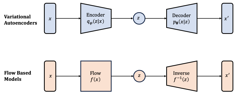
VAEs compress data into a lower-dimensional latent space using an encoder, then reconstruct it with a decoder. Flow-based models use a single invertible transformation that keeps the same dimensionality between input and latent space. This enables exact inference and likelihood computation.
To understand how normalizing flows enable exact likelihood computation, we first need to explore a fundamental mathematical concept: the change-of-variable formula. This principle lies at the heart of flow models, allowing us to transform probability densities through invertible functions. We’ll begin with the 1D case and build up to the multivariate formulation.
2 Math Review
This section builds the mathematical foundation for understanding flow models, starting with change-of-variable and extending to multivariate transformations and Jacobians.
2.1 Change of Variables in 1D
Suppose we have a random variable \(z\) with a known distribution \(p_Z(z)\), and we define a new variable:
\[ x = f(z) \]
where \(f\) is a monotonic, differentiable function with an inverse:
\[ z = f^{-1}(x) = h(x) \]
Our goal is to compute the probability density function (PDF) of \(x\), denoted \(p_X(x)\), in terms of the known PDF \(p_Z(z)\).
2.1.1 Cumulative Distribution Function (CDF)
We begin with the cumulative distribution function of \(x\):
\[ F_X(x) = P(X \leq x) = P(f(Z) \leq x) \]
Since \(f\) is monotonic and invertible, this becomes:
\[ P(f(Z) \leq x) = P(Z \leq f^{-1}(x)) = F_Z(h(x)) \]
2.1.2 Deriving the PDF via Chain Rule
To obtain the PDF, we differentiate the CDF:
\[ p_X(x) = \frac{d}{dx} F_X(x) = \frac{d}{dx} F_Z(h(x)) \]
Applying the chain rule:
\[ p_X(x) = F_Z'(h(x)) \cdot h'(x) = p_Z(h(x)) \cdot h'(x) \]
2.1.3 Rewrite in Terms of \(z\)
From the previous step:
\[ p_X(x) = p_Z(h(x)) \cdot h'(x) \]
Since \(z = h(x)\), we can rewrite:
\[ p_X(x) = p_Z(z) \cdot h'(x) \]
Now, using the inverse function theorem, we express \(h'(x)\) as:
\[ h'(x) = \frac{d}{dx} f^{-1}(x) = \frac{1}{f'(z)} \]
So the final expression becomes:
\[ p_X(x) = p_Z(z) \cdot \left| \frac{1}{f'(z)} \right| \]
The absolute value ensures the density remains non-negative, as required for any valid probability distribution.
This is the fundamental concept normalizing flows use to model complex distributions by transforming simple ones.
2.2 Geometry: Determinants and Volume Changes
To further understand the multivariate change-of-variable formula, it’s helpful to first explore how linear transformations affect volume in high-dimensional spaces.
Let \(\mathbf{Z}\) be a random vector uniformly distributed in the unit cube \([0,1]^n\), and let \(\mathbf{X} = A\mathbf{Z}\), where \(A\) is a square, invertible matrix. Geometrically, the matrix \(A\) maps the unit hypercube to a parallelogram in 2D or a parallelotope in higher dimensions.
The determinant of a square matrix tells us how the transformation scales volume. For instance, if the determinant of a \(2 \times 2\) matrix is 3, applying that matrix will stretch the area of a region by a factor of 3. A negative determinant indicates a reflection, meaning the transformation also flips the orientation. When measuring volume, we care about the absolute value of the determinant.
The volume of the resulting parallelotope is given by:
\[ \text{Volume} = |\det(A)| \]
This expression tells us how much the transformation \(A\) scales space. For example, if \(|\det(A)| = 2\), the transformation doubles the volume.
To make this idea concrete, consider the illustration below. The left figure shows a uniform distribution over the unit square \([0, 1]^2\). When we apply the linear transformation \(A = \begin{bmatrix} a & b \\ c & d \end{bmatrix}\), each point in the square is mapped to a new location, stretching the square into a parallelogram. The area of this parallelogram — and hence the volume scaling — is given by the absolute value of the determinant \(|\det(A)| = |ad - bc|\).
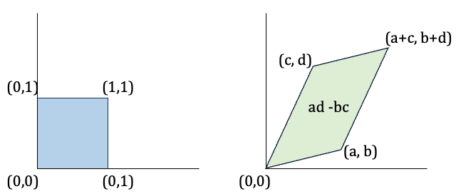
A linear transformation maps a unit square to a parallelogram.
This geometric intuition becomes essential when we apply the same logic to probability densities. The area of the parallelogram equals the absolute value of the determinant, |det(A)|, indicating how the transformation scales area.
2.3 Determinants and Probability Density
Previously, we saw how a linear transformation scales volume. Now we apply the same idea to probability densities — since density is defined per unit volume, scaling the volume also affects the density.
To transform the density from \(\mathbf{Z}\) to \(\mathbf{X}\), we use the change-of-variable formula. Since \(\mathbf{X} = A\mathbf{Z}\), the inverse transformation is \(\mathbf{Z} = A^{-1} \mathbf{X}\). This tells us how to evaluate the density at \(\mathbf{x}\) by “pulling it back” through the inverse mapping. Applying the multivariate change-of-variable rule:
\[ p_X(\mathbf{x}) = p_Z(W \mathbf{x}) \cdot \left| \det(W) \right| \quad \text{where } W = A^{-1} \]
This is directly analogous to the 1D change-of-variable rule:
\[ p_X(x) = p_Z(h(x)) \cdot |h'(x)| \]
but now in multiple dimensions using the determinant of the inverse transformation.
To make this more concrete, here’s a simple 2D example demonstrating how linear transformations affect probability density.
Let \(\mathbf{Z}\) be a random vector uniformly distributed over the unit square \([0, 1]^2\). Suppose we apply the transformation \(\mathbf{X} = A\mathbf{Z}\), where
\[ A = \begin{bmatrix} 2 & 0 \\ 0 & 1 \end{bmatrix} \quad \text{so that} \quad W = A^{-1} = \begin{bmatrix} \frac{1}{2} & 0 \\ 0 & 1 \end{bmatrix} \]
This transformation stretches the square horizontally, doubling its width while keeping the height unchanged. As a result, the area is doubled:
\[
|\det(A)| = 2 \quad \text{and} \quad |\det(W)| = \frac{1}{2}
\] Since the same total probability must be spread over a larger area, the density decreases, meaning the probability per unit area is reduced due to the increased area over which the same total probability is distributed.
Now, let’s say \(p_Z(z) = 1\) inside the unit square (a uniform distribution). To compute \(p_X(\mathbf{x})\) at a point \(\mathbf{x}\) in the transformed space, we use:
\[ p_X(\mathbf{x}) = p_Z(W\mathbf{x}) \cdot |\det(W)| = 1 \cdot \frac{1}{2} = \frac{1}{2} \]
So, the transformed density is halved — the same total probability (which must remain 1) is now spread over an area that is twice as large.
2.4 Generalizing to Nonlinear Transformations
For nonlinear transformations \(\mathbf{x} = f(\mathbf{z})\), the idea is similar. But instead of a constant matrix \(A\), we now consider the Jacobian matrix of the function \(f\):
\[ J_f(\mathbf{z}) = \frac{\partial f}{\partial \mathbf{z}} \]
The Jacobian matrix generalizes derivatives to multivariable functions, capturing how a transformation scales and rotates space locally through all partial derivatives. Its determinant tells us how much the transformation stretches or compresses space — acting as a local volume scaling factor.
2.5 Multivariate Change-of-Variable
Given an invertible transformation \(\mathbf{x} = f(\mathbf{z})\), the probability density transforms as:
\[ p_X(\mathbf{x}) = p_Z(f^{-1}(\mathbf{x})) \cdot \left| \det \left( \frac{\partial f^{-1}(\mathbf{x})}{\partial \mathbf{x}} \right) \right| \]
Alternatively, in the forward form (often used during training):
\[ p_X(\mathbf{x}) = p_Z(\mathbf{z}) \cdot \left| \det \left( \frac{\partial f(\mathbf{z})}{\partial \mathbf{z}} \right) \right|^{-1} \]
This generalizes the 1D rule and enables us to compute exact likelihoods for complex distributions as long as the transformation is invertible and differentiable. This formula is pivotal in machine learning, where transformations of probability distributions are common — such as in the implementation of normalizing flows for generative modeling.
3 Flow Model
A normalizing flow model defines a one-to-one and reversible transformation between observed variables \(\mathbf{x}\) and latent variables \(\mathbf{z}\). This transformation is given by an invertible, differentiable function \(f_\theta\), parameterized by \(\theta\):
\[ \mathbf{x} = f_\theta(\mathbf{z}) \quad \text{and} \quad \mathbf{z} = f_\theta^{-1}(\mathbf{x}) \]
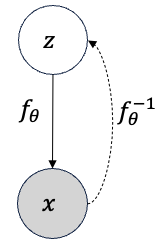
Flow model showing forward and inverse transformations
Figure: A flow-based model uses a forward transformation \(f_\theta\) to map from latent variables (\(\mathbf{z}\)) to data (\(\mathbf{x}\)), and an inverse transformation \(f_\theta^{-1}\) to compute likelihoods. Adapted from class notes (XCS236, Stanford).
Because the transformation is invertible, we can apply the change-of-variable formula to compute the exact probability of \(\mathbf{x}\):
\[ p_X(\mathbf{x}; \theta) = p_Z(f_\theta^{-1}(\mathbf{x})) \cdot \left| \det \left( \frac{\partial f_\theta^{-1}(\mathbf{x})}{\partial \mathbf{x}} \right) \right| \]
This makes it possible to evaluate exact likelihoods and learn the model via maximum likelihood estimation (MLE).
Note: Both \(\mathbf{x}\) and \(\mathbf{z}\) must be continuous and have the same dimensionality since the transformation must be invertible.
3.1 Model Architecture: A Sequence of Invertible Transformations
The term flow refers to the fact that we can compose multiple invertible functions to form a more expressive transformation:
\[ \mathbf{z}_m = f_\theta^{(m)} \circ f_\theta^{(m-1)} \circ \cdots \circ f_\theta^{(1)}(\mathbf{z}_0) \]
In this setup:
- \(\mathbf{z}_0 \sim p_Z\) is sampled from a simple base distribution (e.g., standard Gaussian)
- \(\mathbf{x} = \mathbf{z}_M\) is the final transformed variable
- The full transformation \(f_\theta\) is the composition of \(M\) sequential invertible functions. Each function slightly reshapes the distribution, and together they produce a highly expressive mapping from a simple base distribution to a complex one.
The visuals below illustrate this idea from two angles. The first diagram illustrates the structure of a normalizing flow as a composition of invertible steps, while the second shows how this architecture reshapes simple distributions into complex ones through repeated transformations.

Adapted from Wikipedia: Mapping simple distributions to complex ones via invertible transformations.
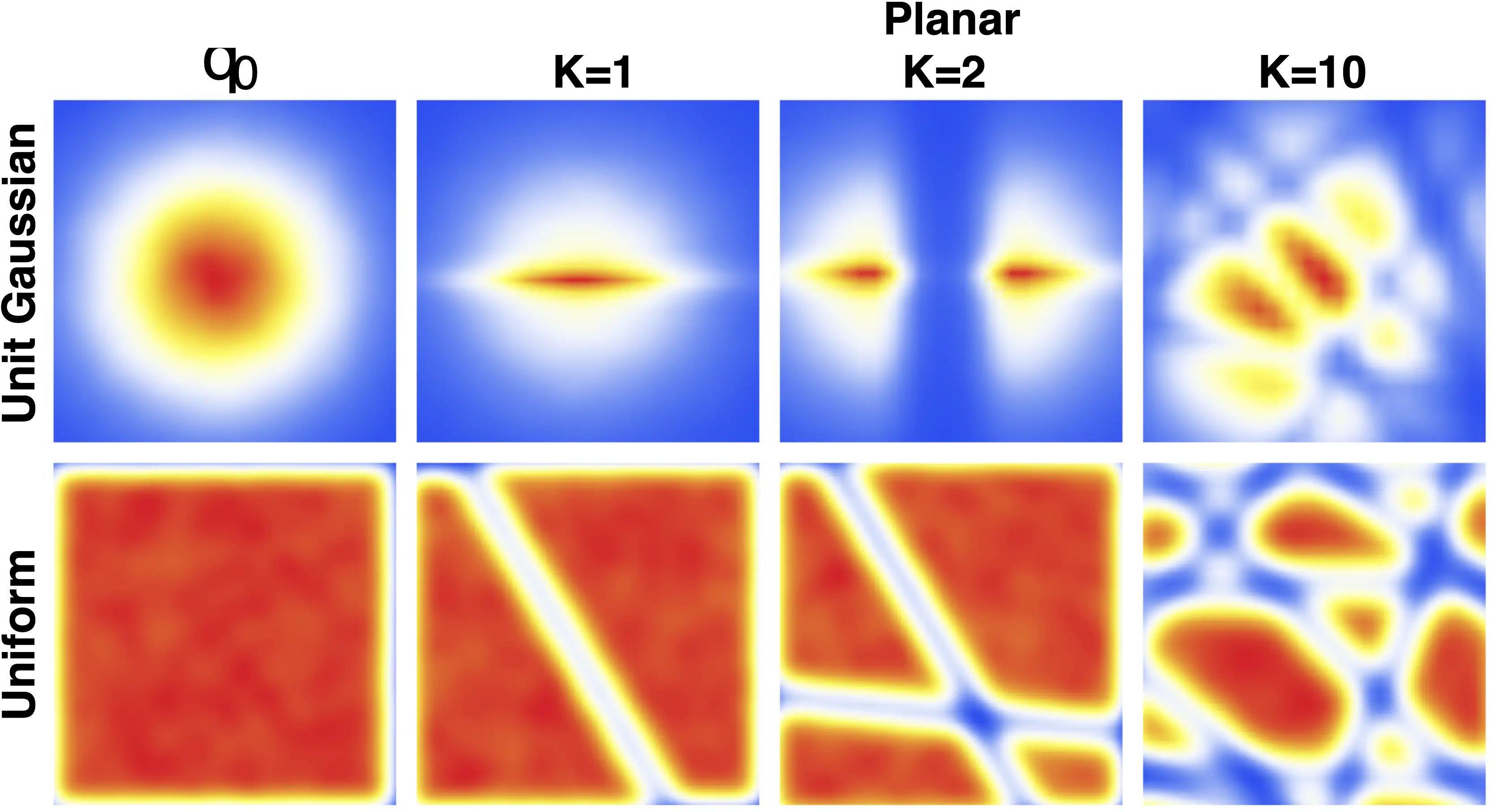
Adapted from class notes (XCS236, Stanford), originally based on Rezende & Mohamed, 2016.
The density of \(\mathbf{x}\) is given by the change-of-variable formula:
\[ p_X(\mathbf{x}; \theta) = p_Z(f_\theta^{-1}(\mathbf{x})) \cdot \prod_{m=1}^M \left| \det \left( \frac{\partial (f_\theta^{(m)})^{-1}(\mathbf{z}_m)}{\partial \mathbf{z}_m} \right) \right| \]
This approach allows the model to approximate highly complex distributions using simple building blocks.
4 Learning and Inference
Training a flow-based model is done by maximizing the log-likelihood over the dataset \(\mathcal{D}\):
\[ \max_\theta \log p_X(\mathcal{D}; \theta) = \sum_{\mathbf{x} \in \mathcal{D}} \log p_Z(f_\theta^{-1}(\mathbf{x})) + \log \left| \det \left( \frac{\partial f_\theta^{-1}(\mathbf{x})}{\partial \mathbf{x}} \right) \right| \]
Key advantages of normalizing flows:
- Exact likelihoods: No approximation needed — just apply the change-of-variable rule
- Efficient sampling: Generate new data by drawing \(\mathbf{z} \sim p_Z\) and computing \(\mathbf{x} = f_\theta(\mathbf{z})\)
- Latent inference: Invert \(f_\theta\) to compute latent codes \(\mathbf{z} = f_\theta^{-1}(\mathbf{x})\), without needing a separate encoder
4.1 Computational Considerations
One challenge in training normalizing flow models is that computing the exact likelihood requires evaluating the determinant of the Jacobian matrix of the transformation:
- For a transformation \(f : \mathbb{R}^n \to \mathbb{R}^n\), the Jacobian is an \(n \times n\) matrix.
- Computing its determinant has a cost of \(\mathcal{O}(n^3)\), which is computationally expensive during training — especially in high dimensions.
4.1.1 Key Insight
To make normalizing flows scalable, we design transformations where the Jacobian has a special structure that makes the determinant easy to compute.
For example: - If the Jacobian is a triangular matrix, the determinant is just the product of the diagonal entries, which can be computed in \(\mathcal{O}(n)\) time. - This works because in a triangular matrix, all the off-diagonal elements are zero — so the determinant simplifies significantly.
In practice, flow models like RealNVP and MAF are designed so that each output dimension \(x_i\) depends only on some subset of the input dimensions \(z_{\leq i}\) (for lower triangular structure) or \(z_{\geq i}\) (for upper triangular structure). This results in a Jacobian of the form:
\[ J = \frac{\partial \mathbf{f}}{\partial \mathbf{z}} = \begin{pmatrix} \frac{\partial f_1}{\partial z_1} & 0 & \cdots & 0 \\ \ast & \frac{\partial f_2}{\partial z_2} & \cdots & 0 \\ \vdots & \vdots & \ddots & \vdots \\ \ast & \ast & \cdots & \frac{\partial f_n}{\partial z_n} \end{pmatrix} \]
Because of this triangular structure, computing the determinant becomes as simple as multiplying the diagonal terms:
\[ \det(J) = \prod_{i=1}^{n} \frac{\partial f_i}{\partial z_i} \]
This is why many modern flow models rely on coupling layers or autoregressive masking: they preserve invertibility and enable efficient, exact likelihood computation.
5 Types of Flow Architectures
This section introduces common architectural families used in normalizing flows, highlighting their core ideas, strengths, and limitations.
5.1 Elementwise Flows
- Idea: Apply a simple invertible function to each variable independently.
- Examples: Leaky ReLU, Softplus, ELU.
- Strengths: Extremely fast; easy to implement; analytically tractable.
- Limitations: Cannot model interactions or dependencies between variables.
5.2 Linear Flows
- Idea: Apply a linear transformation using an invertible matrix (e.g., permutation, rotation, LU decomposition).
- Examples: Glow’s 1x1 Convolution, LU flows.
- Strengths: Efficiently models global dependencies; can be used to permute variables.
- Limitations: Limited expressiveness when used alone.
5.3 Coupling Flows
- Idea: Split the input into two parts. One half remains unchanged while the other is transformed based on it.
- Examples: NICE (additive), RealNVP (affine).
- Strengths: Easy to invert and compute Jacobians; scalable to high dimensions.
- Limitations: Requires stacking multiple layers to mix information across all dimensions.
5.4 Autoregressive Flows
- Idea: Model the transformation of each variable conditioned on the previous ones in a fixed order.
- Examples: Masked Autoregressive Flow (MAF), Inverse Autoregressive Flow (IAF).
- Strengths: Highly expressive; models arbitrary dependencies.
- Limitations: Slower sampling or density evaluation depending on flow direction.
5.5 Residual Flows
- Idea: Add residual connections while enforcing invertibility (e.g., using constraints on Jacobian eigenvalues).
- Examples: Planar flows, Radial flows, Residual Flows (Behrmann et al.).
- Strengths: Flexible and capable of complex transformations.
- Limitations: May require care to ensure invertibility; harder to train.
5.6 Continuous Flows
- Idea: Model the transformation as the solution to a differential equation parameterized by a neural network.
- Examples: Neural ODEs, FFJORD.
- Strengths: Highly flexible; enables continuous-time modeling.
- Limitations: Computationally expensive; uses ODE solvers during training and inference.
These architectures can be mixed and matched in real-world models to balance expressiveness, efficiency, and tractability. Each comes with trade-offs, and their selection often depends on the task and data at hand.
In the rest of this article, we focus on Coupling Flows, briefly introducing NICE and then diving deeper into the structure, intuition, and implementation details of RealNVP.
5.7 NICE: Nonlinear Independent Components Estimation
The NICE (Nonlinear Independent Components Estimation) model, introduced by Laurent Dinh, David Krueger, and Yoshua Bengio in 2014, is a foundational work in the development of normalizing flows.
It provides a framework for transforming complex high-dimensional data into a simpler latent space (often a standard Gaussian), enabling both exact likelihood estimation and sampling — two fundamental goals in generative modeling.
5.7.1 Core Concepts
Invertible Transformations:
NICE constructs a chain of invertible functions to map inputs to latent variables. This ensures that both the forward and inverse transformations are tractable.Additive Coupling Layers:
The model partitions the input into two parts and applies an additive transformation to one part using a function of the other. This design yields a triangular Jacobian with determinant 1, making log-likelihood computation efficient.Volume-Preserving Mapping:
Because additive coupling layers do not scale the space, NICE preserves volume — i.e., the Jacobian determinant is exactly 1. While this limits expressiveness, it simplifies training and inference.Scaling Layer (Optional):
The original NICE paper includes an optional scaling layer at the end to allow some volume change per dimension.Exact Log-Likelihood:
Unlike VAEs or GANs, which rely on approximations, NICE enables exact evaluation of the log-likelihood, making it a fully probabilistic, likelihood-based model.
5.7.2 Additive Coupling Layer
To make the transformation invertible and computationally efficient, NICE splits the input vector into two parts. One part is kept unchanged, while the other part is modified using a function of the unchanged part. This way, we can easily reverse the process because we always know what was kept intact.
Let’s partition the input \(\mathbf{z} \in \mathbb{R}^n\) into two subsets: \(\mathbf{z}_{1:d}\) and \(\mathbf{z}_{d+1:n}\) for some \(1 \leq d < n\).
- Forward Mapping \(\mathbf{z} \mapsto \mathbf{x}\):
\[ \begin{aligned} \mathbf{x}_{1:d} &= \mathbf{z}_{1:d} \quad \text{(identity transformation)} \\ \mathbf{x}_{d+1:n} &= \mathbf{z}_{d+1:n} + m_\theta(\mathbf{z}_{1:d}) \end{aligned} \]
where \(m_\theta(\cdot)\) is a neural network with parameters \(\theta\), \(d\) input units, and \(n - d\) output units.
- Inverse Mapping \(\mathbf{x} \mapsto \mathbf{z}\):
\[ \begin{aligned} \mathbf{z}_{1:d} &= \mathbf{x}_{1:d} \quad \text{(identity transformation)} \\ \mathbf{z}_{d+1:n} &= \mathbf{x}_{d+1:n} - m_\theta(\mathbf{x}_{1:d}) \end{aligned} \]
- Jacobian of the forward mapping:
The Jacobian matrix captures how much the transformation stretches or compresses space. Because the unchanged subset passes through as-is and the transformation is purely additive (no scaling), the Jacobian is triangular with 1s on the diagonal — so its determinant is 1 — meaning the transformation preserves volume.
\[ J = \frac{\partial \mathbf{x}}{\partial \mathbf{z}} = \begin{pmatrix} I_d & 0 \\ \frac{\partial m_\theta}{\partial \mathbf{z}_{1:d}} & I_{n-d} \end{pmatrix} \]
\[ \det(J) = 1 \]
Hence, additive coupling is a volume-preserving transformation.
5.7.3 Rescaling Layer
To overcome the limitation of fixed volume, NICE adds a diagonal scaling transformation at the end, allowing the model to contract or expand space. This is not part of the coupling layers, but is crucial to increase flexibility.
- Forward Mapping:
\[ x_i = s_i z_i \quad \text{with} \quad s_i > 0 \]
- Inverse Mapping:
\[ z_i = \frac{x_i}{s_i} \]
- Jacobian:
\[ J = \text{diag}(\mathbf{s}) \quad \Rightarrow \quad \det(J) = \prod_{i=1}^n s_i \]
However, the volume-preserving property of NICE limits its expressiveness. RealNVP extends this idea by introducing affine coupling layers that enable volume changes during transformation.
5.8 Real-NVP: Non-Volume Preserving Extension of NICE
Real-NVP (Dinh et al., 2017) extends NICE by introducing a scaling function that allows the model to change volume, enabling more expressive transformations. This is achieved using affine coupling layers that apply learned scaling and translation functions to part of the input while keeping the rest unchanged.
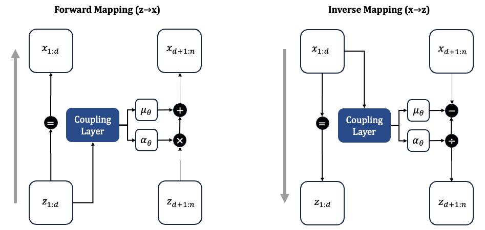
Visualization of a single affine coupling layer in RealNVP. The identity path and affine transform structure allow exact inversion and efficient computation.
We partition the input \(\mathbf{z} \in \mathbb{R}^n\) into two subsets: \(\mathbf{z}_{1:d}\) and \(\mathbf{z}_{d+1:n}\).
- Forward Mapping \(\mathbf{z} \mapsto \mathbf{x}\):
\[ \begin{aligned} \mathbf{x}_{1:d} &= \mathbf{z}_{1:d} \quad \text{(identity transformation)} \\\\ \mathbf{x}_{d+1:n} &= \mathbf{z}_{d+1:n} \odot \exp(\alpha_\theta(\mathbf{z}_{1:d})) + \mu_\theta(\mathbf{z}_{1:d}) \end{aligned} \]
Here, \(\boldsymbol{\alpha}_\theta(\cdot)\) and \(\boldsymbol{\mu}_\theta(\cdot)\) are neural networks with parameters \(\theta\) that take the unchanged subset \(\mathbf{z}_{1:d}\) as input and produce scale and shift parameters, respectively, for the transformed subset \(\mathbf{z}_{d+1:n}\). These functions enable flexible, learnable affine transformations while preserving invertibility.
- Inverse Mapping \(\mathbf{x} \mapsto \mathbf{z}\):
\[ \begin{aligned} \mathbf{z}_{1:d} &= \mathbf{x}_{1:d} \quad \text{(identity transformation)} \\\\ \mathbf{z}_{d+1:n} &= \left( \mathbf{x}_{d+1:n} - \mu_\theta(\mathbf{x}_{1:d}) \right) \odot \exp(-\alpha_\theta(\mathbf{x}_{1:d})) \end{aligned} \]
The inverse mapping recovers the latent variable \(\mathbf{z}\) from the data \(\mathbf{x}\). The first subset \(\mathbf{x}_{1:d}\) remains unchanged and directly becomes \(\mathbf{z}_{1:d}\). To reconstruct \(\mathbf{z}_{d+1:n}\), we first subtract the shift \(\boldsymbol{\mu}_\theta(\mathbf{x}_{1:d})\) from \(\mathbf{x}_{d+1:n}\), and then apply an elementwise rescaling using \(\exp(-\boldsymbol{\alpha}_\theta(\mathbf{x}_{1:d}))\). This inversion relies on the same neural networks used in the forward pass and ensures that the transformation is exactly reversible.
- Jacobian of Forward Mapping:
\[ J = \frac{\partial \mathbf{x}}{\partial \mathbf{z}} = \begin{pmatrix} I_d & 0 \\\\ \frac{\partial \mathbf{x}_{d+1:n}}{\partial \mathbf{z}_{1:d}} & \operatorname{diag}\left(\exp(\alpha_\theta(\mathbf{z}_{1:d}))\right) \end{pmatrix} \]
The Jacobian matrix of the RealNVP forward transformation has a special block structure due to the design of the affine coupling layer:
Upper left block: \(\mathbf{I}_d\)
This corresponds to the partial derivatives of \(\mathbf{x}_{1:d}\) with respect to \(\mathbf{z}_{1:d}\). Since the first \(d\) variables are passed through unchanged (\(\mathbf{x}_{1:d} = \mathbf{z}_{1:d}\)), their derivatives form an identity matrix.Upper right block: \(0\)
These derivatives are zero because \(\mathbf{x}_{1:d}\) does not depend on \(\mathbf{z}_{d+1:n}\) at all — they’re completely decoupled.Lower right block: (diagonal)
Each element of \(\mathbf{x}_{d+1:n}\) is scaled elementwise by \(\exp\left(\left[\alpha_\theta(\mathbf{z}_{1:d})\right]_i\right)\). This means the Jacobian of this part is a diagonal matrix, where each diagonal entry is the corresponding scale factor.Lower left block:
This part can contain non-zero values because \(\mathbf{x}_{d+1:n}\) depends on \(\mathbf{z}_{1:d}\) via the neural networks. But thanks to the triangular structure of the Jacobian, we don’t need this block to compute the determinant.
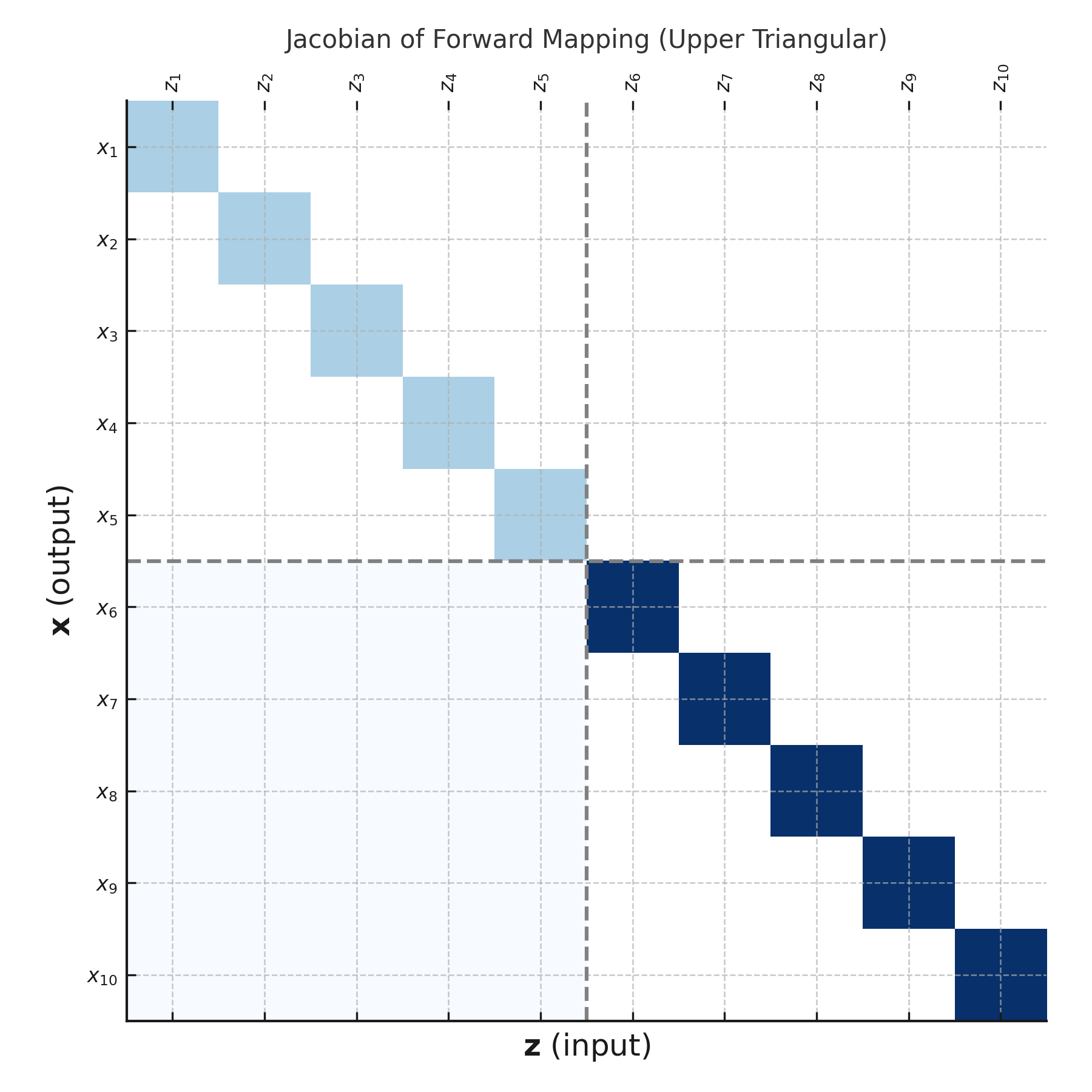
Jacobian of the RealNVP forward transformation. Upper triangular structure arises because the first subset is unchanged, while the second is scaled and shifted based on the first.
5.8.1 Why This Structure Matters
Because the Jacobian is triangular, its determinant is simply the product of the diagonal entries.
\[ \det(J) = \prod_{i=d+1}^{n} \exp\left( \alpha_\theta(\mathbf{z}_{1:d})_i \right) = \exp\left( \sum_{i=d+1}^{n} \alpha_\theta(\mathbf{z}_{1:d})_i \right) \]
In log-space, this becomes a sum:
\[ \log \det(J) = \sum_{i=d+1}^{n} \alpha_\theta(\mathbf{z}_{1:d})_i \]
This makes the computation of log-likelihoods fast and tractable.
Taking the product of the diagonal entries gives us a measure of how much the transformation expands or contracts local volume. If the determinant is greater than 1, the transformation expands space; if it’s less than 1, it contracts space. Since the determinant is not fixed, RealNVP performs a non-volume preserving transformation — allowing it to model more complex distributions than NICE, which preserves volume by design.
5.8.2 Stacking Coupling Layers
Each coupling layer only transforms part of the input. To ensure that every dimension is eventually updated, RealNVP stacks multiple coupling layers and alternates the masking pattern between them.
- In one layer, the first half is fixed, and the second half is transformed.
- In the next layer, the roles are reversed.
This alternating structure ensures: - All input dimensions are updated across layers - The full transformation remains invertible - The total log-determinant is the sum of the log-determinants of each layer
5.8.3 RealNVP in Action (Two Moons)
The following plots illustrate how RealNVP transforms data in practice:

Top-left: Original two-moons data (X)
Top-right: Encoded latent space (Z) Bottom-left: Latent samples from base distribution
Bottom-right: Generated samples mapped back to (X) space
5.8.4 Summary
To recap the key distinctions between NICE and RealNVP, here’s a side-by-side comparison:
| Aspect | NICE | RealNVP |
|---|---|---|
| Type of coupling | Additive | Affine (scaling + shift) |
| Volume change | Only possible with rescaling layer | Built into each coupling layer |
| Jacobian determinant | 1 (in coupling layers) | Varies (depends on learned scale) |
| Expressiveness | Limited (volume-preserving layers) | Higher (learns scale & shift) |
| Log-likelihood | Exact | Exact |
6 🧪 Try It Yourself: Flow Model in Pytorch
You can explore a minimal PyTorch implementation of a normalizing flow model:
7 References
[1] Stanford CS236 Notes. “Normalizing Flows”
[2] UT Austin Calculus Notes. “Jacobian and Change of Variables”
[3] Danilo Jimenez Rezende, and Shakir Mohamed. “Variational Inference with Normalizing Flows”
[4] Kobyzev, Prince, and Brubaker. “Normalizing Flows: An Introduction and Review of Current Methods”
[5] Wikipedia. “Normalizing Flow”
8 Further Reading
[1] George Papamakarios et al. “Normalizing Flows for Probabilistic Modeling and Inference”
[2] Lilian Weng. “Flow-based Models”
[3] Eric Jang. “Normalizing Flows Tutorial – Part 1”
[4] Eric Jang. “Normalizing Flows Tutorial – Part 2”